- Setup
- 1. How real models turn probabilities into text
- 2. The plan
- 3. Batches
- 4. The loss, smoothed
- 5. The optimizer and the learning rate
- 6. Half precision
- 7. Training
- 8. Decoding by search
- 9. Decoding by sampling
- 10. Inside the trained model
- 11. Next to a real translator
- 12. Save and publish
- References
Transformers: from scratch to production · lesson 3 of 9 · all lessons · run on Kaggle · open in Colab · code on GitHub
Ask a chatbot the same question twice and you may get two different answers. Ask a translation model twice and you get the same translation both times. The networks inside are close relatives, so the difference isn’t in the model. It is in the step after it: every model of this kind produces probabilities for the next token, and a separate procedure, decoding, turns those probabilities into text. Here is how four real models are shipped to decode, read from their own configuration files:
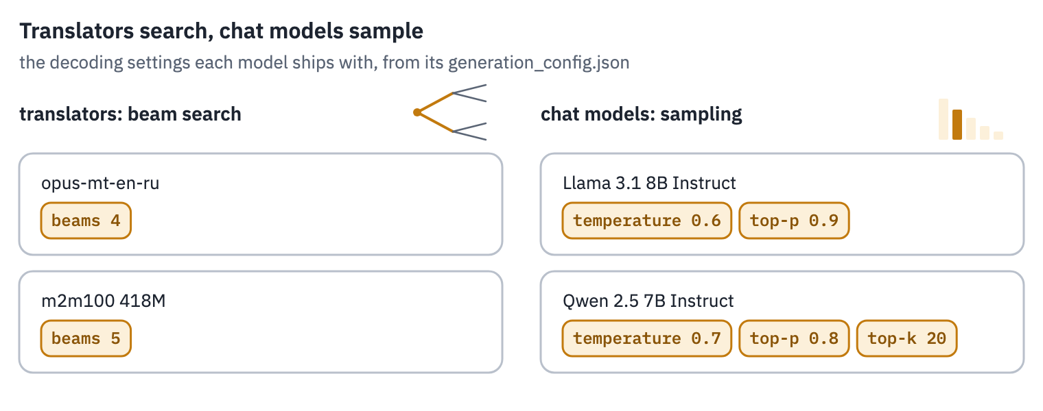
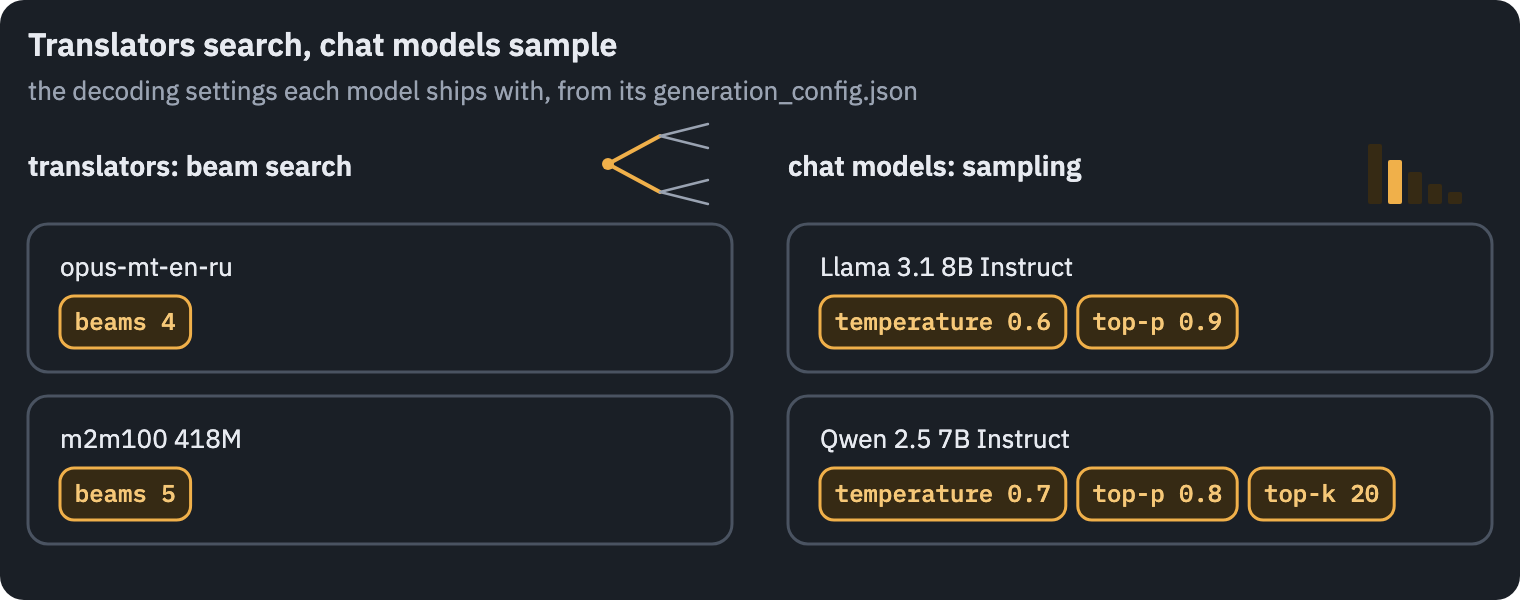
The translators search for the most probable sentence; the chat models sample, drawing each next token at random from its probabilities. By the end of this lesson you’ll have written both, and seen why each side chose its way.
First the model has to have probabilities worth decoding. In lesson 2 our Transformer could only parrot the token it had just read, or recite sixteen sentences it had learned by heart. In this lesson it trains on half a million sentence pairs, on a free GPU, in about twenty minutes, with the recipe of the 2017 paper: batches built from tokens, a smoothed loss, Adam with a warm-up, and half-precision arithmetic. Every piece is explained and tested before it goes into the loop.
What you’ll do
- Turn half a million pairs into batches that waste little on padding.
- Build the training step: label smoothing, Adam with the paper’s learning-rate schedule, gradient clipping, mixed precision. See what warm-up is for by training without it.
- Train the lesson 2 Transformer and watch it go from parrot to translator, epoch by epoch.
- Decode three ways: greedy, beam search and sampling.
- Look inside: does сказала now look at she? And put our model next to opus-mt-en-ru.
What you need: a GPU. On Kaggle, Settings → Accelerator → GPU; on Colab, Runtime → Change runtime type → T4 GPU. The notebook downloads lesson 1’s data and tokenizer and imports lesson 2’s model. It runs in under an hour.
Setup
One small helper package, tfs, draws the course’s plots and token chips and knows where the notebook runs (Kaggle, Colab or your own machine). Everything the lesson teaches is written out in the notebook itself.
import importlib.util
import subprocess
import sys

TFS = "git+https://github.com/xmarva/transformers-from-scratch@main"
if importlib.util.find_spec("tfs") is None:
    subprocess.check_call([sys.executable, "-m", "pip", "install", "-q", TFS])

from tfs import env
from tfs.viz import table, token_chips, use_course_style

env.quiet()  # no progress bars or environment warnings in the outputs
SEED = 42
env.seed_everything(SEED)
COLORS = use_course_style()
WORK_DIR = env.work_dir()
import json
import math
import os
import random
import time

import matplotlib.pyplot as plt
import numpy as np
import pandas as pd
import torch
import torch.nn.functional as F
from huggingface_hub import HfApi, hf_hub_download
from tfs.model import Transformer
from tfs.viz import heatmap
from tokenizers import Tokenizer

SMOKE = env.smoke()  # CI runs the lesson on a tiny slice; you train in full
device = "cuda" if torch.cuda.is_available() else "cpu"
assert device == "cuda" or SMOKE, "This lesson trains a model: switch to a GPU (see above)."
if device == "cuda":
    print("GPU:", torch.cuda.get_device_name(0))
GPU: Tesla T4The data and the tokenizer of lesson 1, from the Hugging Face Hub:
tokenizer_path = hf_hub_download("xmarva/tfs-bpe-en-ru-16k", "tokenizer.json")
tokenizer = Tokenizer.from_file(tokenizer_path)

splits = {}
for name in ["train", "validation", "test"]:
    path = hf_hub_download(
        "xmarva/tfs-tatoeba-en-ru", f"data/{name}.parquet", repo_type="dataset"
    )
    splits[name] = pd.read_parquet(path)
train, valid, test = splits["train"], splits["validation"], splits["test"]

VOCAB_SIZE = tokenizer.get_vocab_size()
PAD = tokenizer.token_to_id("<pad>")
BOS = tokenizer.token_to_id("<bos>")
EOS = tokenizer.token_to_id("<eos>")
print("train:", len(train), "validation:", len(valid), "test:", len(test))
train: 508093 validation: 10370 test: 363851. How real models turn probabilities into text
A model like ours never outputs a sentence. At every step it outputs one probability for each token of its vocabulary, given the source sentence and everything written so far. Here is opus-mt-en-ru, the translator we will compete with in lesson 4, writing our sentence:
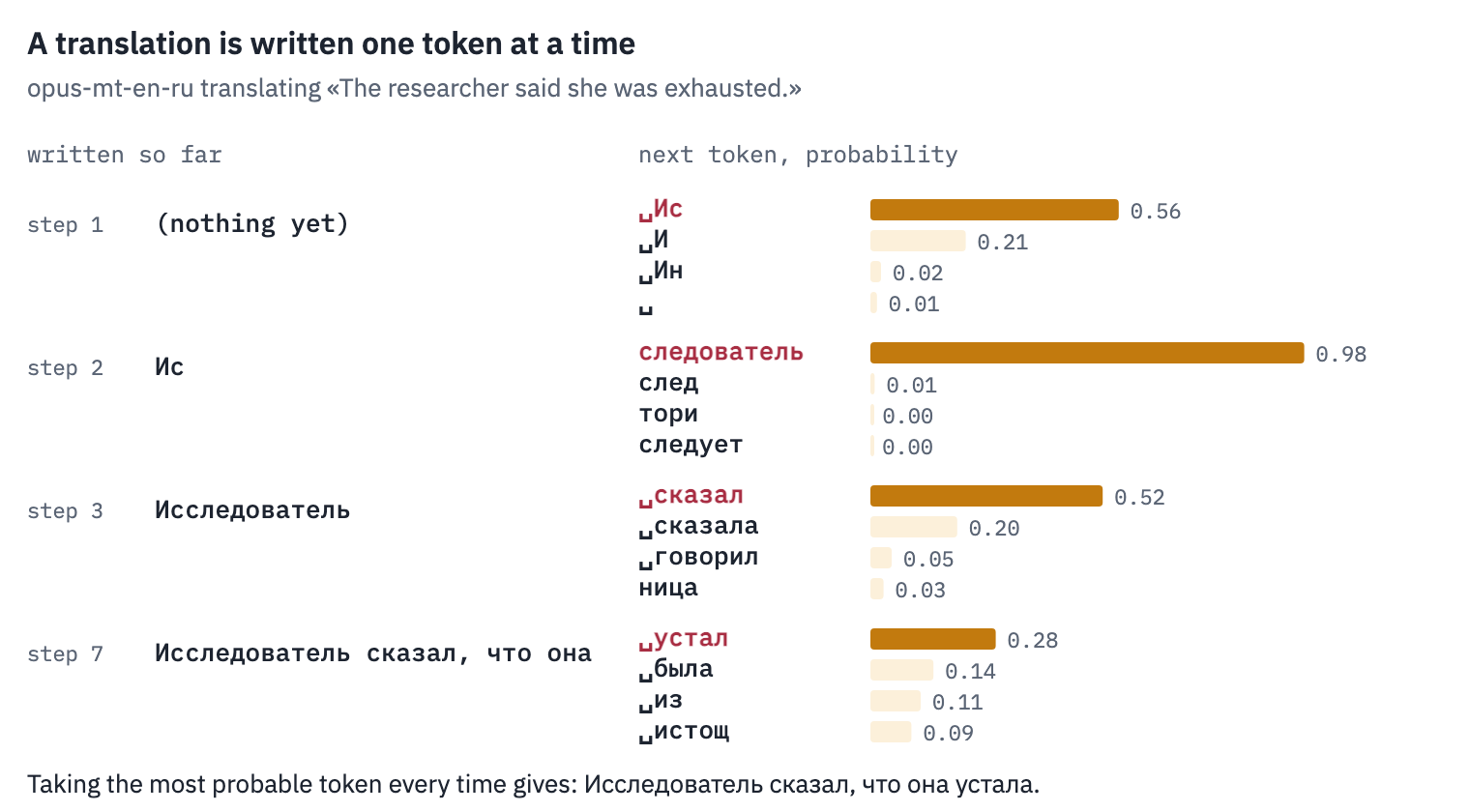
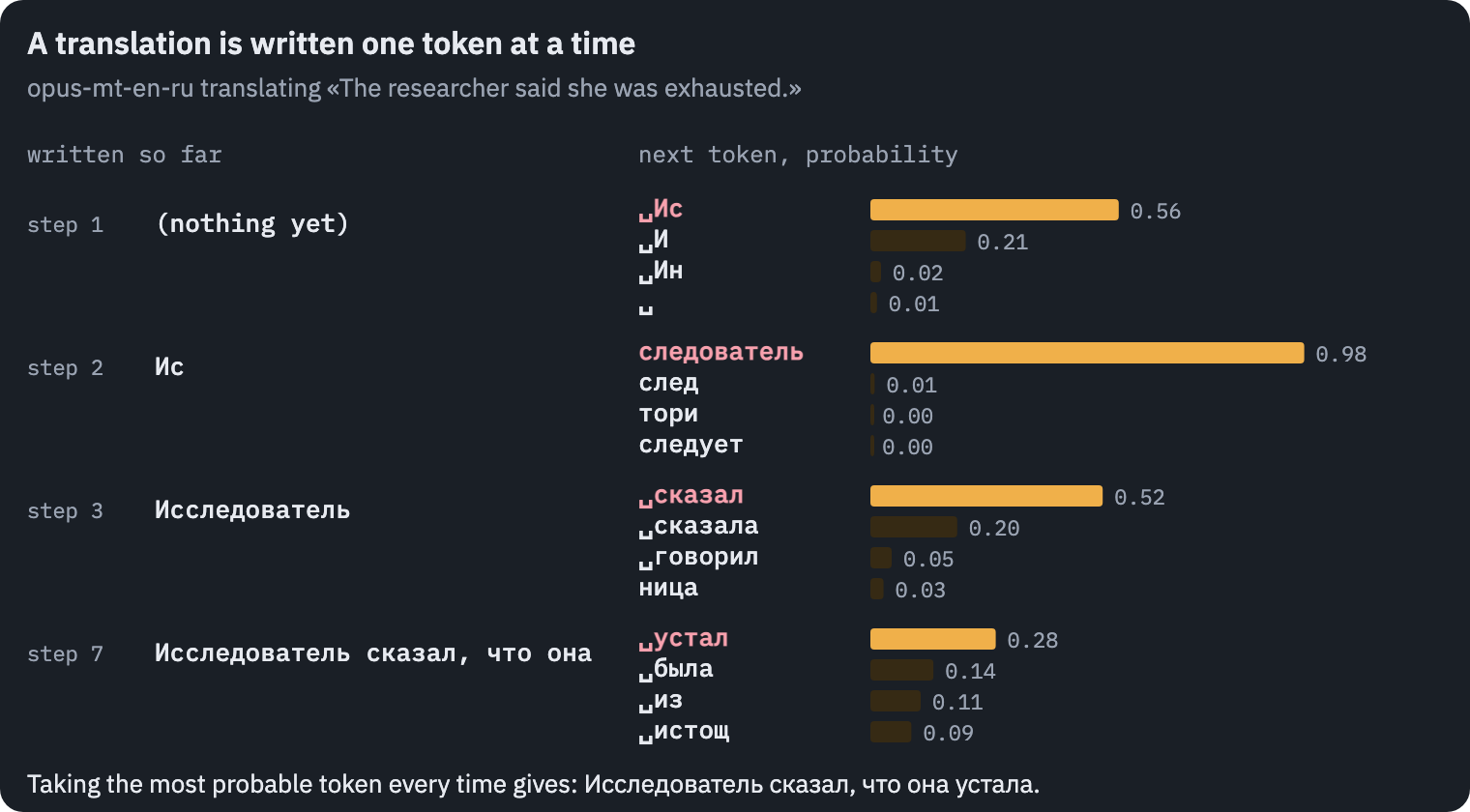
Some steps are easy: after Ис, the continuation следователь gets almost all of the probability. Others are real choices. At the verb, the model gives the masculine сказал about half of it and the feminine сказала a fifth; it even keeps a small chance for ница, the suffix that would make the researcher a woman. The model itself doesn’t choose; it hands these numbers on. Which token gets written is decided by a separate procedure, decoding, and the picture used the simplest one: take the most probable token at every step. That’s how the masculine translation of section 8 comes about.
A model on the Hugging Face Hub can come with a generation_config.json: the decoding settings its authors recommend. Read four of them, two translators and two chat models:
GENERATION_CONFIGS = {
    "opus-mt-en-ru (translator)": "Helsinki-NLP/opus-mt-en-ru",
    "m2m100 418M (translator)": "facebook/m2m100_418M",
    "Llama 3.1 8B Instruct (chat)": "unsloth/Meta-Llama-3.1-8B-Instruct",
    "Qwen 2.5 7B Instruct (chat)": "Qwen/Qwen2.5-7B-Instruct",
}

rows = []
for name, repo in GENERATION_CONFIGS.items():
    with open(hf_hub_download(repo, "generation_config.json")) as f:
        config = json.load(f)
    rows.append(
        {
            "model": name,
            "beams": config.get("num_beams", 1),
            "samples": config.get("do_sample", False),
            "temperature": config.get("temperature", "–"),
            "top-p": config.get("top_p", "–"),
        }
    )
table(pd.DataFrame(rows))
| model | beams | samples | temperature | top-p |
|---|---|---|---|---|
| opus-mt-en-ru (translator) | 4 | False | – | – |
| m2m100 418M (translator) | 5 | False | – | – |
| Llama 3.1 8B Instruct (chat) | 1 | True | 0.60 | 0.90 |
| Qwen 2.5 7B Instruct (chat) | 1 | True | 0.70 | 0.80 |
The two translators keep 4 and 5 beams: candidate translations followed in parallel, so that the model can choose the most probable whole sentence rather than the most probable next word. The chat models instead sample with a temperature below 1 and a top-p cut-off, settings that control how adventurous the random choice is. Sections 8 and 9 build all of this. Behind the difference is a different idea of a good output: a translation has to be faithful, an answer in a conversation has to be varied and alive.
2. The plan
Training repeats one step thousands of times. Each piece of this loop is a section of the lesson:
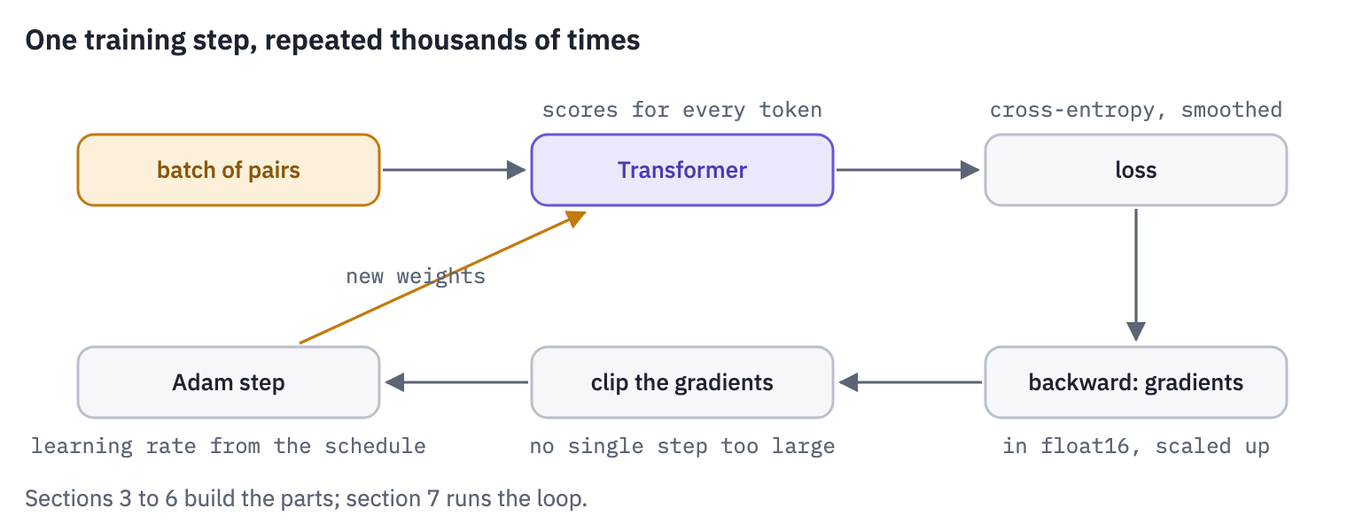
In words: take a batch of sentence pairs, let the model score every possible next token at every position, measure how far the scores are from the right answers (the loss), compute how each weight should change to reduce it (the gradients, by backpropagation), and move every weight a small step in that direction. The size of the step is the learning rate, and how it changes over training is the schedule.
3. Batches
The GPU reads the data in batches, and the first decision is what a batch is. Start by turning every sentence into token ids once, so that the training loop never touches text. encode_batch runs the Rust tokenizer on many sentences in parallel:
if SMOKE:
    train = train.sample(3_000, random_state=SEED)
    valid = valid.head(300)


def encode_all(sentences):
    return [encoding.ids for encoding in tokenizer.encode_batch(list(sentences))]


start = time.perf_counter()
train_src, train_tgt = encode_all(train.en), encode_all(train.ru)
valid_src, valid_tgt = encode_all(valid.en), encode_all(valid.ru)
seconds = round(time.perf_counter() - start, 1)
print("tokenized", len(train_src) + len(valid_src), "pairs in", seconds, "s")
tokenized 518463 pairs in 35.7 sHow long are the sentences, in tokens?
en_lengths = [len(ids) for ids in train_src]
ru_lengths = [len(ids) for ids in train_tgt]

fig, ax = plt.subplots(figsize=(6.4, 3))
bins = np.arange(0, max(en_lengths + ru_lengths) + 2)
ax.hist(en_lengths, bins=bins, color=COLORS["enc"], alpha=0.6, label="English")
ax.hist(ru_lengths, bins=bins, histtype="step", color=COLORS["dec"], label="Russian")
ax.set_yscale("log")  # to see the rare long sentences next to the common short ones
ax.set_xlabel("tokens per sentence")
ax.set_ylabel("sentences")
ax.set_title("Tatoeba sentences are short")
ax.legend()
plt.show()

print("longest English:", max(en_lengths), "tokens; longest Russian:", max(ru_lengths))
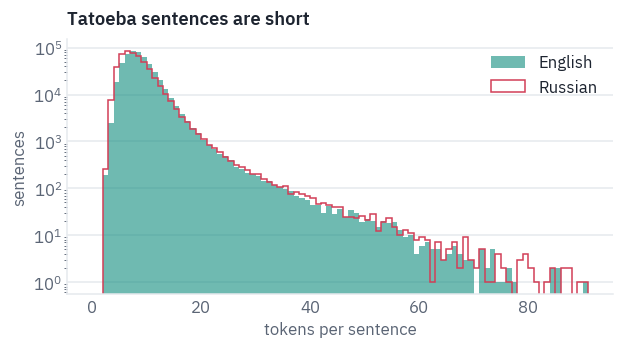
longest English: 90 tokens; longest Russian: 90Most sentences take a handful of tokens (mind the logarithmic scale), and a thin tail of long ones reaches far to the right. That tail matters for the GPU. In a batch every sentence is padded to the longest one, and a padded position costs as much as a real one, so a single long sentence would turn the rest of its batch into mostly padding. We leave out the few pairs longer than 64 tokens on either side:
MAX_LEN = 64

keep = []
for i in range(len(train_src)):
    if len(train_src[i]) <= MAX_LEN and len(train_tgt[i]) + 1 <= MAX_LEN:  # +1: <bos>/<eos>
        keep.append(i)
print("training pairs kept:", len(keep), "of", len(train_src))
training pairs kept: 508021 of 508093Now the batches. A fixed number of sentences per batch would make the batches of long sentences much more expensive than the others, so the size of a batch is measured in tokens: a batch takes sentences until it would exceed MAX_TOKENS positions, padding included. And because padding is wasted work, it matters which sentences share a batch. Compare a random batch with a batch of sentences of similar length; violet cells are real tokens, grey ones padding:
def pad_batch(sequences):
    longest = max(len(ids) for ids in sequences)
    batch = torch.full((len(sequences), longest), PAD)
    for row, ids in enumerate(sequences):
        batch[row, : len(ids)] = torch.tensor(ids)
    return batch


by_length = sorted(keep, key=lambda i: len(train_tgt[i]))  # shortest Russian first
examples = {
    "random": random.sample(keep, 12),
    "similar lengths": by_length[len(by_length) // 2 :][:12],  # 12 pairs from the middle
}

for name, rows_of_batch in examples.items():
    batch = pad_batch([train_tgt[i] for i in rows_of_batch])
    padding = (batch == PAD).float().mean().item()
    title = f"A {name} batch: {padding:.0%} padding"
    heatmap(batch != PAD, low="grid", cell=0.18, title=title)
plt.show()
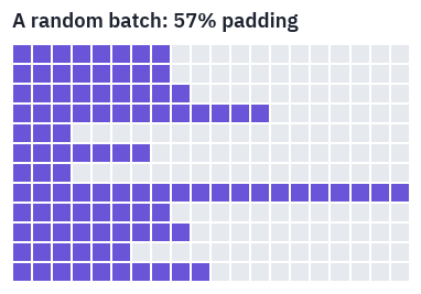
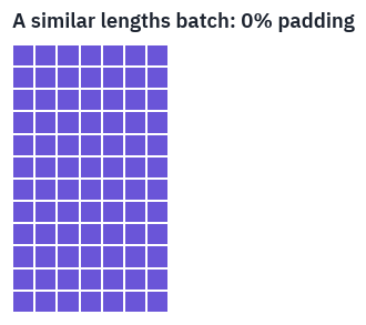
The standard fix is bucketing: sort the pairs by length, cut the sorted list into batches, and shuffle the order of the batches, so that the model still sees a random mix of lengths over an epoch while every single batch is nearly free of padding. make_batches does exactly that and builds the three tensors a training step needs, as in lesson 2: the English ids, the Russian ids behind <bos> that the decoder reads, and the Russian ids followed by <eos> that it must predict.
def make_batches(src, tgt, rows, max_tokens, sort=True):
    if sort:
        # similar lengths side by side
        rows = sorted(rows, key=lambda i: (len(tgt[i]), len(src[i])))
    batches, current, longest = [], [], 0
    for i in rows:
        new_longest = max(longest, len(src[i]), len(tgt[i]) + 1)
        if current and new_longest * (len(current) + 1) > max_tokens:  # the batch is full
            batches.append(current)
            current, new_longest = [], max(len(src[i]), len(tgt[i]) + 1)
        current.append(i)
        longest = new_longest
    batches.append(current)

    tensors = []
    for batch in batches:
        src_ids = pad_batch([src[i] for i in batch])
        tgt_in = pad_batch([[BOS] + tgt[i] for i in batch])
        tgt_out = pad_batch([tgt[i] + [EOS] for i in batch])
        tensors.append((src_ids, tgt_in, tgt_out))
    return tensors


def padding_share(batches):
    real, total = 0, 0
    for src_ids, _, tgt_out in batches:
        real += int((src_ids != PAD).sum() + (tgt_out != PAD).sum())
        total += src_ids.numel() + tgt_out.numel()
    return 1 - real / total


MAX_TOKENS = 6_000  # positions per batch and side, padding included

train_batches = make_batches(train_src, train_tgt, keep, MAX_TOKENS)
valid_batches = make_batches(valid_src, valid_tgt, range(len(valid_src)), MAX_TOKENS)
print("training batches:", len(train_batches), "validation batches:", len(valid_batches))
print(f"padding in the bucketed batches: {padding_share(train_batches):.1%}")
training batches: 814 validation batches: 22
padding in the bucketed batches: 1.8%
Little padding left. For comparison, the same token budget with the pairs in random order:
random_rows = random.sample(keep, len(keep))
unsorted = make_batches(train_src, train_tgt, random_rows, MAX_TOKENS, sort=False)
print(f"padding in random batches: {padding_share(unsorted):.1%}")
print("random batches:", len(unsorted), "bucketed:", len(train_batches))
del unsorted  # only needed for the comparison
padding in random batches: 70.6%
random batches: 2733 bucketed: 814
Random batches waste a large share of every step on padding, and need more steps to cover the same data. One trade-off of bucketing: a batch now holds sentences of one length, so its gradient is a little less representative of the whole data than a random batch’s. Shuffling the batch order every epoch keeps that harmless in practice, and the paper’s authors batched the same way.
4. The loss, smoothed
The loss is the cross-entropy of lesson 2. At every position the model turns its scores \(\mathbf{z}\) into probabilities with softmax, \(p_j = e^{z_j} / \sum_k e^{z_k}\), and pays \(-\log p_y\), where \(y\) is the right token:
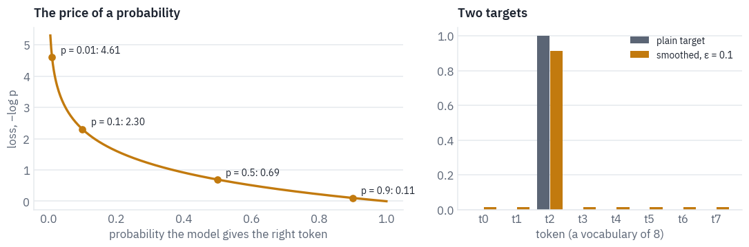
\[\mathcal{L} = -\log p_y.\]Read \(-\log p\) as surprise. A model that gave the right token probability 1 isn’t surprised at all and pays 0; one that gave it 0.5 pays 0.69; one that was confident in something else and gave the right token 0.01 pays 4.6, and the price grows without bound as \(p_y \to 0\). Averaged over all target tokens of a batch, this is the number training brings down.
Written as a sum over the vocabulary, the same loss compares the model’s distribution \(p\) with a target distribution \(q\) that puts all its mass on the right token:
\[\mathcal{L} = -\sum_{j=1}^{\lvert\mathcal{V}\rvert} q_j \log p_j, \qquad q_j = \begin{cases} 1 & j = y \\ 0 & \text{otherwise.} \end{cases}\]That target is a demand for certainty. On data like ours, where He’s stupid. has two dozen correct translations (lesson 1), total certainty is wrong anyway. Label smoothing (Szegedy et al., 2016), used in the 2017 paper with \(\varepsilon = 0.1\), softens the target: it keeps \(1 - \varepsilon\) of the mass on the right token and spreads \(\varepsilon\) evenly over the whole vocabulary,
\[q_j = (1 - \varepsilon)\,[j = y] + \frac{\varepsilon}{\lvert\mathcal{V}\rvert}.\]Both ideas in one picture: the price of a probability, and the two targets, drawn here for a vocabulary of eight tokens so that the spread part is visible (in ours, each of sixteen thousand tokens gets \(\varepsilon / 16\,000\)):
EPSILON = 0.1

fig, axes = plt.subplots(1, 2, figsize=(10, 3.4), gridspec_kw={"width_ratios": [1.3, 1]})

ax = axes[0]
p_right = np.linspace(0.005, 1, 400)
ax.plot(p_right, -np.log(p_right), color=COLORS["data"])
for p_value in [0.9, 0.5, 0.1, 0.01]:
    surprise = -math.log(p_value)
    ax.plot(p_value, surprise, "o", color=COLORS["data"])
    ax.annotate(f"p = {p_value}: {surprise:.2f}", (p_value, surprise), xytext=(8, 4),
                textcoords="offset points", fontsize=9)
ax.set_xlabel("probability the model gives the right token")
ax.set_ylabel("loss, −log p")
ax.set_title("The price of a probability")

ax = axes[1]
tokens = np.arange(8)
one_hot = np.zeros(8)
one_hot[2] = 1  # token 2 is the right one
smoothed = (1 - EPSILON) * one_hot + EPSILON / 8
ax.bar(tokens - 0.2, one_hot, width=0.38, color=COLORS["muted"], label="plain target")
label = f"smoothed, ε = {EPSILON}"
ax.bar(tokens + 0.2, smoothed, width=0.38, color=COLORS["data"], label=label)
ax.set_xticks(tokens, [f"t{k}" for k in tokens])
ax.set_xlabel("token (a vocabulary of 8)")
ax.set_title("Two targets")
ax.legend(fontsize=9)
plt.tight_layout()
plt.show()
Why does the target matter so much? Because of the gradient. Differentiate the loss with respect to the scores and almost everything cancels:
\[\frac{\partial \mathcal{L}}{\partial z_j} = p_j - q_j.\]Training moves every score in proportion to how far the model’s probability is from the target: the right token’s score goes up by \(1 - p_y\) at most, every other score goes down by its own probability. With the plain target the push on the right token only stops at \(p_y = 1\), which needs its score infinitely far above the rest. With the smoothed target the push stops at \(p = q\): the model is rewarded for being mostly sure. The paper reports that this hurts perplexity, since the model learns to be less sure, but improves the translations.
Check both formulas, the loss and its gradient, against PyTorch on five tokens, small enough to follow:
scores = torch.tensor([[2.0, 0.5, -1.0, 0.0, 1.0]], requires_grad=True)  # one position
right = torch.tensor([0])  # the right token is token 0

q = torch.full((1, 5), EPSILON / 5)  # spread epsilon evenly...
q[0, 0] += 1 - EPSILON  # ...and keep the rest on the right token

p = scores.softmax(dim=-1)
ours = -(q * p.log()).sum()
theirs = F.cross_entropy(scores, right, label_smoothing=EPSILON)
assert torch.allclose(ours, theirs)

theirs.backward()  # the gradient of PyTorch's loss with respect to the scores
assert torch.allclose(scores.grad, p - q)

print("target q:      ", q)
print("probabilities: ", p.detach().round(decimals=4))
print("gradient p - q:", scores.grad.round(decimals=4))
print("loss:", round(ours.item(), 4), "= PyTorch's", round(theirs.item(), 4))
target q:       tensor([[0.9200, 0.0200, 0.0200, 0.0200, 0.0200]])
probabilities:  tensor([[0.5630, 0.1256, 0.0280, 0.0762, 0.2071]])
gradient p - q: tensor([[-0.3570,  0.1056,  0.0080,  0.0562,  0.1871]])
loss: 0.7244 = PyTorch's 0.7244
The right token’s gradient is negative, so training raises its score; the four others are positive and go down.
One consequence to remember when reading the training curves: with a smoothed target the loss can’t reach zero. Its minimum is reached when \(p = q\), and then it equals the entropy of \(q\) itself:
q_right = 1 - EPSILON + EPSILON / VOCAB_SIZE
q_other = EPSILON / VOCAB_SIZE
floor = -(q_right * math.log(q_right) + (VOCAB_SIZE - 1) * q_other * math.log(q_other))
print("lowest possible smoothed loss:", round(floor, 3))
lowest possible smoothed loss: 1.293That’s why we will watch two different numbers: the smoothed loss the model trains on, which levels off above this floor, and the plain cross-entropy on the validation set, which is what we actually want to be low.
5. The optimizer and the learning rate
Gradient descent, and what the learning rate does
The gradient \(\nabla \mathcal{L}(\theta)\) points in the direction in which the loss grows fastest. Gradient descent takes a step the other way, of a size set by the learning rate \(\eta\):
\[\theta \leftarrow \theta - \eta\, \nabla \mathcal{L}(\theta).\]How large can \(\eta\) be? The simplest loss already answers it. Take one weight and a parabola, \(\mathcal{L}(\theta) = \tfrac{\lambda}{2}\theta^2\), whose curvature \(\lambda\) says how steep it is. Its gradient is \(\lambda\theta\), so one step gives
\[\theta_{t+1} = \theta_t - \eta\lambda\theta_t = (1 - \eta\lambda)\,\theta_t.\]Every step multiplies the distance to the minimum by \(1 - \eta\lambda\). If \(0 < \eta\lambda < 1\) the weight creeps towards the minimum from one side; between 1 and 2 it jumps over it and back, closer each time; at \(\eta\lambda > 2\) every jump overshoots by more than the last, and training diverges. Four learning rates on a parabola with \(\lambda = 1\):
def descend(eta, curvature=1.0, start=3.0, n_steps=8):
    theta = start
    path = [theta]
    for _ in range(n_steps):
        gradient = curvature * theta
        theta = theta - eta * gradient
        path.append(theta)
    return np.array(path)


grid = np.linspace(-5, 5, 200)
fig, axes = plt.subplots(1, 4, figsize=(11, 2.8), sharey=True)
for ax, eta in zip(axes, [0.1, 0.6, 1.6, 2.1]):
    path = descend(eta)
    shown = path[np.abs(path) <= 5]  # a diverging path leaves the picture: draw what fits
    ax.plot(grid, grid**2 / 2, color=COLORS["grid"], linewidth=3)
    ax.plot(shown, shown**2 / 2, "-o", color=COLORS["enc"], markersize=4, linewidth=1.2)
    factor = 1 - eta  # 1 - eta * curvature, with curvature 1
    shown_factor = f"{factor:.1f}".replace("-", "−")  # a typographic minus
    if factor < 0:
        shown_factor = f"({shown_factor})"
    verdict = "diverges" if abs(factor) > 1 else "converges"
    ax.set_title(f"η = {eta}: ×{shown_factor} per step, {verdict}", fontsize=10)
    ax.set_xticks([])
axes[0].set_ylabel("loss")
plt.tight_layout()
plt.show()

for eta in [0.1, 0.6, 1.6, 2.1]:
    distance = abs(descend(eta)[-1])
    print(f"η = {eta}: {distance:.2f} from the minimum after 8 steps, starting from 3")
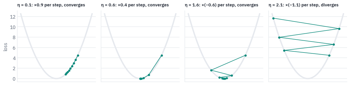
η = 0.1: 1.29 from the minimum after 8 steps, starting from 3
η = 0.6: 0.00 from the minimum after 8 steps, starting from 3
η = 1.6: 0.05 from the minimum after 8 steps, starting from 3
η = 2.1: 6.43 from the minimum after 8 steps, starting from 3
A real loss has millions of directions, each with its own curvature, and one learning rate for all of them. The steepest direction caps it: beyond \(\eta = 2 / \lambda_{\max}\) that direction diverges. The flattest direction then moves by only a factor \(1 - \eta\lambda_{\min}\) per step, which is barely below 1 when the two curvatures are far apart. Here is a valley 100 times steeper across than along, \(\mathcal{L}(\theta) = \tfrac12(100\,\theta_1^2 + \theta_2^2)\), where any \(\eta\) above \(2/100 = 0.02\) diverges.
Adam
The optimizer of the 2017 paper, and of nearly every Transformer since, is Adam (Kingma and Ba, 2015). It gives every weight its own effective step size. For each weight it keeps two running averages, of the gradient and of its square:
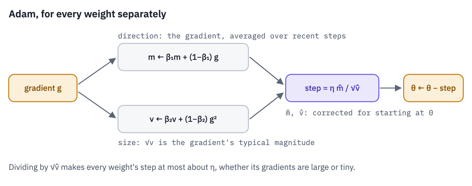
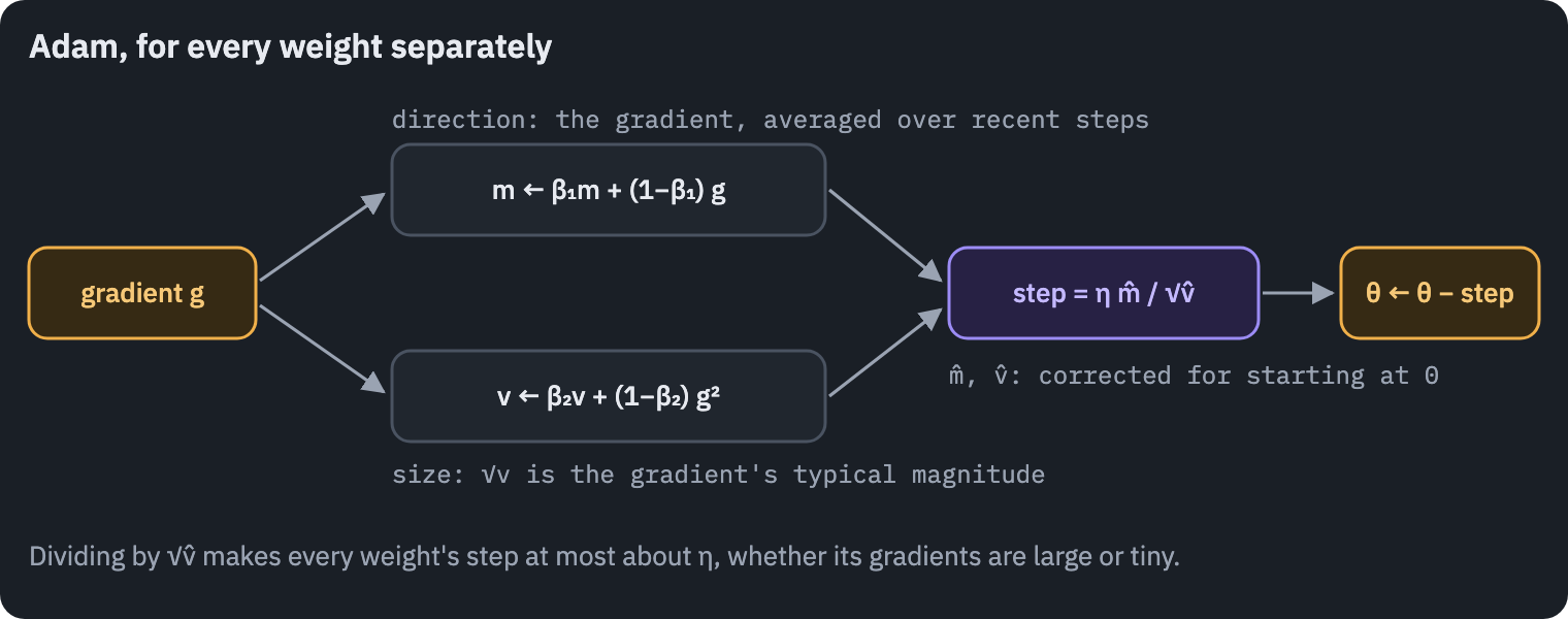
- \(g_t\): the gradient of this weight at step \(t\).
- \(m_t\): its average over roughly the last \(1 / (1 - \beta_1)\) steps. Noise from batch to batch cancels out, and a direction that persists builds up: momentum.
- \(v_t\): the average of its square, so \(\sqrt{v_t}\) is the gradient’s typical magnitude.
- \(\hat m_t, \hat v_t\): both averages start at 0 and would be too small for the first steps; dividing by \(1 - \beta^t\) corrects that, and the correction fades as \(\beta^t \to 0\).
- \(\hat m_t / \sqrt{\hat v_t}\): a gradient measured in units of its own typical size, close to \(\pm 1\) when the gradient is consistent and smaller when it is noisy. So every weight moves by at most about \(\eta\), whether its raw gradients are large or tiny, and the steep and flat directions of the valley move at similar speeds.
- \(\epsilon\): prevents division by zero.
The paper uses \(\beta_1 = 0.9\), \(\beta_2 = 0.98\), \(\epsilon = 10^{-9}\). The update in code, applied to a tensor of weights, is the formula line by line:
def adam_step(theta, gradient, state, step, eta, beta1=0.9, beta2=0.98, eps=1e-9):
    state["m"] = beta1 * state["m"] + (1 - beta1) * gradient
    state["v"] = beta2 * state["v"] + (1 - beta2) * gradient**2
    m_hat = state["m"] / (1 - beta1**step)
    v_hat = state["v"] / (1 - beta2**step)
    return theta - eta * m_hat / (v_hat.sqrt() + eps)
Run it on the valley next to plain gradient descent, and next to PyTorch’s own torch.optim.Adam with the same settings, which must land on exactly the same point:
curvatures = torch.tensor([100.0, 1.0])  # steep across, flat along


def valley_loss(theta):
    return 0.5 * (curvatures * theta**2).sum()


start = torch.tensor([-1.0, 4.0])
n_steps = 60

gradient_descent = [start]
theta = start
for _ in range(n_steps):
    gradient = curvatures * theta  # the gradient of the valley
    theta = theta - 0.019 * gradient  # just below the limit of 0.02
    gradient_descent.append(theta)

adam_path = [start]
theta = start
state = {"m": torch.zeros(2), "v": torch.zeros(2)}
for step in range(1, n_steps + 1):
    theta = adam_step(theta, curvatures * theta, state, step, eta=0.1)
    adam_path.append(theta)

weights = start.clone().requires_grad_()
reference = torch.optim.Adam([weights], lr=0.1, betas=(0.9, 0.98), eps=1e-9)
for _ in range(n_steps):
    reference.zero_grad()
    valley_loss(weights).backward()
    reference.step()
assert torch.allclose(adam_path[-1], weights.detach(), atol=1e-6)
print("adam_step lands where torch.optim.Adam does:", adam_path[-1].tolist())
adam_step lands where torch.optim.Adam does: [0.021380223333835602, -0.09399668872356415]x_grid, y_grid = np.meshgrid(np.linspace(-1.4, 1.4, 200), np.linspace(-1, 4.5, 200))
landscape = 0.5 * (100 * x_grid**2 + y_grid**2)
fig, axes = plt.subplots(1, 2, figsize=(10, 3.8), sharey=True)
paths = [("gradient descent, η = 0.019", gradient_descent), ("Adam, η = 0.1", adam_path)]
for ax, (title, path) in zip(axes, paths):
path = torch.stack(path).numpy()
levels = np.geomspace(0.05, 100, 12) # contour lines of the loss
ax.contour(x_grid, y_grid, landscape, levels=levels, colors=COLORS["grid"])
ax.plot(path[:, 0], path[:, 1], "-o", color=COLORS["enc"], markersize=3, linewidth=1.2)
ax.plot(0, 0, "*", color=COLORS["dec"], markersize=12) # the minimum
final_loss = valley_loss(torch.tensor(path[-1]))
ax.set_title(f"{title}: loss {final_loss:.3f} after {n_steps} steps", fontsize=10)
ax.set_xlabel("θ₁, steep")
ax.grid(False)
axes[0].set_ylabel("θ₂, flat")
plt.tight_layout()
plt.show()
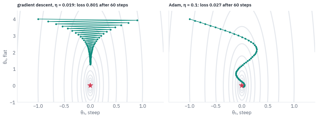
Gradient descent runs at the largest learning rate the steep direction allows. It zigzags across the valley and creeps along it: after sixty steps it is still far up the valley floor. Adam’s steps have about the same length in both directions, so it heads down the valley; its momentum carries it past the minimum and back, in shrinking loops.
The difference grows with the shape of the valley. Make it 25, 100 and 400 times steeper across than along, give gradient descent its best learning rate each time, just below \(2/\lambda_{\max}\), and keep Adam’s \(\eta\) fixed:
def final_point_gradient_descent(curvatures, eta, n_steps=60):
    theta = start
    for _ in range(n_steps):
        theta = theta - eta * curvatures * theta
    return theta


def final_point_adam(curvatures, eta, n_steps=60):
    theta = start
    state = {"m": torch.zeros(2), "v": torch.zeros(2)}
    for step in range(1, n_steps + 1):
        theta = adam_step(theta, curvatures * theta, state, step, eta)
    return theta


rows, adam_points = [], []
for ratio in [25, 100, 400]:
    valley = torch.tensor([float(ratio), 1.0])
    best_eta = 0.95 * 2 / ratio  # 95% of the limit
    descent_point = final_point_gradient_descent(valley, best_eta)
    adam_point = final_point_adam(valley, 0.1)
    adam_points.append(adam_point)
    rows.append(
        {
            "steep / flat": ratio,
            "gradient descent: η": best_eta,
            "loss after 60 steps": 0.5 * (valley * descent_point**2).sum().item(),
            "Adam: loss after 60 steps": 0.5 * (valley * adam_point**2).sum().item(),
        }
    )
table(pd.DataFrame(rows), digits=4)
| steep / flat | gradient descent: η | loss after 60 steps | Adam: loss after 60 steps |
|---|---|---|---|
| 25 | 0.0760 | 0.0006 | 0.0101 |
| 100 | 0.0190 | 0.8007 | 0.0273 |
| 400 | 0.0047 | 4.5187 | 0.0958 |
same_path = all(torch.allclose(point, adam_points[0], atol=1e-5) for point in adam_points)
print("Adam ends at the same point in all three valleys:", same_path)
Adam ends at the same point in all three valleys: TrueOn a mildly uneven valley a well-tuned gradient descent is even ahead. But it falls behind fast as the valley gets more uneven, while Adam ends at exactly the same point in all three. Each coordinate’s gradient is divided by its own typical size, so stretching one direction of the landscape changes nothing for Adam. The loss of a Transformer has millions of directions whose curvatures differ by orders of magnitude, and that is why Adam, not plain gradient descent, trains it.
The learning-rate schedule
The learning rate \(\eta_t\) isn’t constant either. The paper changes it with every step:
\[\eta_t = d_{\text{model}}^{-0.5} \cdot \min\!\big(t^{-0.5},\ t \cdot t_{\text{warm}}^{-1.5}\big).\]For the first \(t_{\text{warm}}\) steps the second term is the smaller one, and the rate grows linearly from zero: the warm-up. After that the first term takes over and the rate decays like \(1/\sqrt{t}\), so the steps get shorter as the model approaches a good solution. The two terms meet at \(t = t_{\text{warm}}\), the peak, and the factor \(d_{\text{model}}^{-0.5}\) makes wider models take smaller steps. Our run lasts EPOCHS passes over the data, one epoch every len(train_batches) steps:
def learning_rate(step, d_model=256, warmup=4_000):
    step = max(step, 1)  # step 0 would divide by zero
    return d_model**-0.5 * min(step**-0.5, step * warmup**-1.5)


WARMUP = 4_000
EPOCHS = 20 if not SMOKE else 1  # the length of the training run in section 7
total_steps = EPOCHS * len(train_batches)

steps = np.arange(1, total_steps + 1)
fig, ax = plt.subplots(figsize=(6.4, 3))
ax.plot(steps, [learning_rate(s, warmup=WARMUP) for s in steps], color=COLORS["enc"])
warmup_end = min(WARMUP, total_steps)
ax.axvspan(0, warmup_end, color=COLORS["enc"], alpha=0.08)
ax.text(warmup_end / 2, 0.0001, "warm-up", ha="center", fontsize=9, color=COLORS["enc"])
for epoch in range(1, EPOCHS + 1):
    ax.axvline(epoch * len(train_batches), color=COLORS["line"], linewidth=0.6)
ax.set_xlabel("step (thin lines: ends of epochs)")
ax.set_ylabel("learning rate")
ax.set_title("Warm up, then decay")
plt.show()

peak = learning_rate(WARMUP, warmup=WARMUP)
print("peak learning rate:", f"{peak:.2e}", "at step", WARMUP)
print("warm-up lasts", round(WARMUP / len(train_batches), 1), "epochs of", EPOCHS)
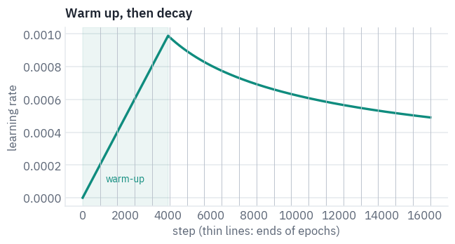
peak learning rate: 9.88e-04 at step 4000
warm-up lasts 4.9 epochs of 20
Why start slowly? At the beginning, Adam’s running average \(v\) has seen only a few gradients, so its estimate of their size is poor and some steps come out far too large (Liu et al., 2020). And a Transformer with normalization after the residual addition, like ours, has especially large gradients near its output at initialization (Xiong et al., 2020). Large early steps can throw the weights somewhere training never recovers from.
Rather than take this on trust, train two copies of the model for a few hundred steps with the same peak learning rate, one with a warm-up and one without. First the pieces of the training step, which section 7 reuses:
CONFIG = {  # the model of lesson 2
    "vocab_size": VOCAB_SIZE,
    "d_model": 256,
    "n_heads": 4,
    "d_ff": 1024,
    "n_layers": 3,
    "dropout": 0.1,
    "pad_id": PAD,
}


def new_model():
    return Transformer(**CONFIG).to(device)


def adam(model):
    # the learning rate is set before every step, from the schedule
    return torch.optim.Adam(model.parameters(), lr=1.0, betas=(0.9, 0.98), eps=1e-9)
The loss of one batch, as in section 4, averaged over all its real target tokens:
def batch_loss(model, batch):
    src_ids, tgt_in, tgt_out = (t.to(device) for t in batch)
    logits = model(src_ids, tgt_in).float()  # the loss in float32 (section 6)
    flat_logits = logits.reshape(-1, VOCAB_SIZE)
    targets = tgt_out.reshape(-1)
    return F.cross_entropy(flat_logits, targets, ignore_index=PAD, label_smoothing=EPSILON)
And the training loop itself: n_steps steps over the batches in shuffled order, each one the picture of section
- It returns the loss of every step.
def train_steps(model, optimizer, schedule, n_steps, first_step=1, use_amp=True, clip=1.0):
    use_amp = use_amp and device == "cuda"
    scaler = torch.amp.GradScaler(device, enabled=use_amp)
    model.train()
    losses = []
    while len(losses) < n_steps:
        order = list(range(len(train_batches)))
        random.shuffle(order)  # a new order on every pass over the data
        for index in order:
            for group in optimizer.param_groups:
                group["lr"] = schedule(first_step + len(losses))

            with torch.autocast(device, dtype=torch.float16, enabled=use_amp):
                loss = batch_loss(model, train_batches[index])

            optimizer.zero_grad()
            scaler.scale(loss).backward()  # gradients of the scaled loss (section 6)
            scaler.unscale_(optimizer)  # back to their true size before clipping
            torch.nn.utils.clip_grad_norm_(model.parameters(), clip)
            scaler.step(optimizer)
            scaler.update()

            losses.append(loss.item())
            if len(losses) == n_steps:
                break
    return losses
train_steps is the loop of the picture in section 2; section 6 explains its lines with autocast and scaler.
One reference point helps to read the experiment: the loss of a model that ignores the sentence altogether and always predicts the same distribution, how often each token occurs in the training targets. A model that has learned nothing more than that sits at this loss:
counts = torch.zeros(VOCAB_SIZE)
for _, _, tgt_out in train_batches:
    counts += torch.bincount(tgt_out[tgt_out != PAD], minlength=VOCAB_SIZE)
frequencies = (counts + 1) / (counts + 1).sum()  # +1 to every count: no probability is 0
log_f = frequencies.log()

# the smoothed loss of always predicting the frequencies:
# 1 - eps of the target on the right token, eps spread evenly over all of them
right_part = -(counts * log_f).sum() / counts.sum()
spread_part = -log_f.mean()
frequency_only = (1 - EPSILON) * right_part + EPSILON * spread_part
frequency_only = frequency_only.item()
print("smoothed loss of predicting only the token frequencies:", round(frequency_only, 2))
smoothed loss of predicting only the token frequencies: 6.96For the experiment, a high peak rate makes the effect easy to see:
PEAK = 3e-3
EXPERIMENT_STEPS = 1_500 if not SMOKE else 10
experiments = {
    "no warm-up": lambda step: PEAK,
    "warm-up over 1 000 steps": lambda step: PEAK * min(1.0, step / 1_000),
}

curves = {}
for name, schedule in experiments.items():
    torch.manual_seed(SEED)  # the same starting weights for both
    model = new_model()
    curves[name] = train_steps(model, adam(model), schedule, EXPERIMENT_STEPS)

fig, ax = plt.subplots(figsize=(6.4, 3.2))
for (name, losses), color in zip(curves.items(), [COLORS["dec"], COLORS["enc"]]):
    smooth = pd.Series(losses).rolling(25, min_periods=1).mean()  # average out the noise
    ax.plot(smooth, color=color, label=name)
ax.axhline(frequency_only, color=COLORS["muted"], linestyle=(0, (3, 3)), linewidth=1)
label = "knows only the token frequencies"
x, y = EXPERIMENT_STEPS * 0.98, frequency_only + 0.45  # above the line, clear of the curves
ax.text(x, y, label, ha="right", va="bottom", fontsize=9)
ax.set_xlabel("step")
ax.set_ylabel("training loss (smoothed)")
ax.set_title("The same peak learning rate, with and without warm-up")
ax.legend()
plt.show()
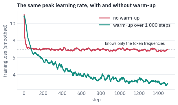
Same model, same data, same peak learning rate; only the first thousand steps differ. With the warm-up, the loss falls steadily. Without it, the first steps at full speed throw the weights somewhere the model doesn’t recover from: the loss sticks near the dashed line, where a model knows little more than which tokens are frequent. In the real run the warm-up lasts longer and the peak is lower, but the reason for it is the one you just saw.
The last protection is gradient clipping, the clip_grad_norm_ line: if the length of the whole gradient vector, over all the model’s weights, exceeds a limit \(c\), the vector is scaled down to that length,
The direction stays, only an occasional huge step is cut short (Pascanu et al., 2013). The 2017 paper doesn’t mention it; it has become a standard part of training recipes since, and \(c = 1\) is a common choice.
6. Half precision
A GPU computes much faster with 16-bit numbers than with the usual 32-bit ones: half the memory traffic, and on the T4 special units (tensor cores) built for 16-bit matrix products. The price is range and precision:
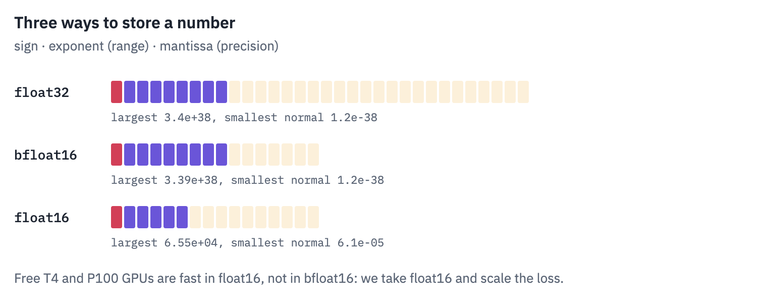
float16 keeps 10 bits of precision, plenty for activations and weights in a matrix product, but only 5 bits of exponent: nothing above 65 504, precision fading below \(2^{-14} \approx 6 \cdot 10^{-5}\), and below \(2^{-24} \approx 6 \cdot 10^{-8}\) nothing but zero. A gradient rounded to zero teaches nothing:
tiny_gradient = torch.tensor(1e-8)
print("in float16:", tiny_gradient.half().item())
print("times 65 536, in float16:", (tiny_gradient * 65_536).half().item())
in float16: 0.0
times 65 536, in float16: 0.0006551742553710938
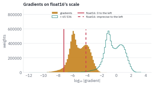
Are real gradients that small? Take the model of the warm-up experiment, after its 1 500 steps, compute the gradients of all its weights on one batch in full float32 precision, and see where they fall on float16’s scale:
model.train()
model.zero_grad()
batch_loss(model, train_batches[0]).backward()
gradients = torch.cat([w.grad.flatten() for w in model.parameters()]).abs().cpu()
gradients = gradients[gradients > 0]  # the logarithm needs positive numbers

SCALE = 2**16
zero_in_float16 = 2.0**-24  # below this, float16 rounds to 0
imprecise_in_float16 = 2.0**-14  # below this, float16 loses precision
fig, ax = plt.subplots(figsize=(6.4, 3.2))
bins = np.linspace(-12, 4, 100)
raw = gradients.log10().numpy()
scaled = (gradients * SCALE).log10().numpy()
ax.hist(raw, bins=bins, color=COLORS["data"], alpha=0.85, label="gradients")
ax.hist(scaled, bins=bins, histtype="step", color=COLORS["enc"], label="× 65 536")
below_legend = 0.68  # the lines stop under the legend
zero = math.log10(zero_in_float16)
ax.axvline(zero, ymax=below_legend, color=COLORS["dec"], label="float16: 0 to the left")
imprecise = math.log10(imprecise_in_float16)
label = "float16: imprecise to the left"
ax.axvline(imprecise, ymax=below_legend, color=COLORS["dec"], ls=(0, (3, 3)), label=label)
ax.set_ylim(top=ax.get_ylim()[1] * 1.45)  # room for the legend above the bars
ax.set_xlabel("log₁₀ |gradient|")
ax.set_ylabel("weights")
ax.set_title("Gradients on float16's scale")
ax.legend(fontsize=8, loc="upper center", ncol=2)
plt.show()
below_zero = (gradients < zero_in_float16).float().mean().item()
below_precise = (gradients < imprecise_in_float16).float().mean().item()
after_scaling = (gradients * SCALE < zero_in_float16).float().mean().item()
print(f"gradients float16 would round to 0:    {below_zero:.2%}")
print(f"gradients where float16 loses precision: {below_precise:.1%}")
print(f"rounded to 0 after scaling by 65 536:  {after_scaling:.4%}")
gradients float16 would round to 0:    4.23%
gradients where float16 loses precision: 74.2%
rounded to 0 after scaling by 65 536:  0.0016%
A few percent of the gradients would vanish outright, and most of them would lose precision. Multiplying the loss by \(2^{16}\) multiplies every gradient by the same factor (the chain rule is linear), shifts the whole histogram to the right and brings almost all of them into range.
That is mixed precision (Micikevicius et al., 2018): matrix products run in float16 under torch.autocast, while the weights and the sensitive operations (softmax, the loss) stay in float32; and loss scaling: multiply the loss by a large factor before backpropagation, then divide the gradients back before the optimizer uses them. GradScaler does both and picks the factor itself: it raises it while all goes well and lowers it, skipping that step, whenever a gradient overflows. In train_steps these are the lines with autocast and scaler.
What does it buy? Time a few steps each way:
TIMING_STEPS = 40 if not SMOKE else 3
timings = {}
for name, use_amp in [("float32", False), ("mixed precision", True)]:
    torch.manual_seed(SEED)
    model = new_model()
    optimizer = adam(model)
    train_steps(model, optimizer, lambda step: 5e-4, 5, use_amp=use_amp)  # warm the GPU up
    if device == "cuda":
        torch.cuda.synchronize()  # wait for the GPU to finish before reading the clock
    start = time.perf_counter()
    train_steps(model, optimizer, lambda step: 5e-4, TIMING_STEPS, use_amp=use_amp)
    if device == "cuda":
        torch.cuda.synchronize()
    timings[name] = (time.perf_counter() - start) / TIMING_STEPS

speedup = timings["float32"] / timings["mixed precision"]
for name, seconds in timings.items():
    print(f"{name}: {seconds * 1000:.0f} ms per step")
print(f"mixed precision is {speedup:.1f} times faster")
float32: 141 ms per step
mixed precision: 69 ms per step
mixed precision is 2.0 times faster
7. Training
Everything is in place. The training run uses the paper’s schedule with a warm-up of WARMUP steps, label smoothing and mixed precision, and after every epoch, one pass over all the batches, it does three things: measures the plain cross-entropy on the validation set, keeps the weights if they are the best so far, and translates a few probe sentences, so that we can watch the model learn.
@torch.no_grad()
def validation_loss(model):
    model.eval()
    total, count = 0.0, 0
    for src_ids, tgt_in, tgt_out in valid_batches:
        src_ids, tgt_in, tgt_out = src_ids.to(device), tgt_in.to(device), tgt_out.to(device)
        with torch.autocast(device, dtype=torch.float16, enabled=device == "cuda"):
            logits = model(src_ids, tgt_in)
        flat = logits.reshape(-1, VOCAB_SIZE).float()
        loss = F.cross_entropy(flat, tgt_out.reshape(-1), ignore_index=PAD, reduction="sum")
        total += loss.item()
        count += int((tgt_out != PAD).sum())
    return total / count  # plain cross-entropy per target token


@torch.no_grad()
def translate_greedy(model, sentence, max_tokens=60):
    model.eval()
    src_ids = torch.tensor([tokenizer.encode(sentence).ids], device=device)
    memory = model.encode(src_ids)
    written = [BOS]
    for _ in range(max_tokens):
        tgt = torch.tensor([written], device=device)
        next_id = model.decode(tgt, memory, src_ids)[0, -1].argmax().item()
        if next_id == EOS:
            break
        written.append(next_id)
    return tokenizer.decode(written[1:])


EN_EXAMPLE = "The researcher said she was exhausted."
PROBES = [EN_EXAMPLE, "Tom forgot to lock the door.", "I can't believe you did that."]
The run: EPOCHS passes over the data with the paper’s schedule. After every epoch the loop measures the validation loss, saves the weights if they are the best so far, and translates the three probe sentences. It prints one line per epoch, with the minutes since the start; this is the long cell of the lesson.
CHECKPOINT = WORK_DIR / "transformer.pt"

torch.manual_seed(SEED)
random.seed(SEED)
model = new_model()
optimizer = adam(model)

def schedule(step):
    return learning_rate(step, warmup=WARMUP)


history = []
best = float("inf")
steps_done = 0
start = time.perf_counter()
for epoch in range(1, EPOCHS + 1):
    n_steps = len(train_batches)  # one epoch
    losses = train_steps(model, optimizer, schedule, n_steps, first_step=steps_done + 1)
    steps_done += len(losses)

    record = {
        "epoch": epoch,
        "step": steps_done,
        "training loss": float(np.mean(losses)),
        "validation loss": validation_loss(model),
        "minutes": (time.perf_counter() - start) / 60,
    }
    for probe in PROBES:
        record[probe] = translate_greedy(model, probe)
    history.append(record)

    if record["validation loss"] < best:
        best = record["validation loss"]
        torch.save(model.state_dict(), CHECKPOINT)
    print(
        f"epoch {epoch:2d}  training {record['training loss']:.3f}  "
        f"validation {record['validation loss']:.3f}  {record['minutes']:.1f} min"
    )
epoch  1  training 6.488  validation 4.497  0.9 min
epoch  2  training 4.501  validation 2.912  1.9 min
epoch  3  training 3.514  validation 2.137  2.9 min
epoch  4  training 3.008  validation 1.724  3.8 min
epoch  5  training 2.754  validation 1.550  4.7 min
epoch  6  training 2.582  validation 1.424  5.7 min
epoch  7  training 2.447  validation 1.292  6.6 min
epoch  8  training 2.351  validation 1.237  7.6 min
epoch  9  training 2.283  validation 1.189  8.5 min
epoch 10  training 2.228  validation 1.169  9.5 min
epoch 11  training 2.185  validation 1.157  10.4 min
epoch 12  training 2.149  validation 1.134  11.4 min
epoch 13  training 2.117  validation 1.114  12.3 min
epoch 14  training 2.092  validation 1.109  13.3 min
epoch 15  training 2.068  validation 1.091  14.2 min
epoch 16  training 2.047  validation 1.075  15.2 min
epoch 17  training 2.029  validation 1.083  16.1 min
epoch 18  training 2.013  validation 1.084  17.0 min
epoch 19  training 1.998  validation 1.067  18.0 min
epoch 20  training 1.984  validation 1.063  18.9 min
The validation loss is a cross-entropy, and its exponent has a readable meaning, the perplexity: the model is as unsure about the next token, on average, as if it were choosing uniformly among that many.
print("best validation loss:", round(best, 3))
print("perplexity:", round(math.exp(best), 2))
best validation loss: 1.063
perplexity: 2.9
history_table = pd.DataFrame(history)
epochs = history_table.epoch
fig, ax = plt.subplots(figsize=(6.4, 3.4))
training, validation = history_table["training loss"], history_table["validation loss"]
ax.plot(epochs, training, marker="o", color=COLORS["enc"], label="training, smoothed")
ax.plot(epochs, validation, marker="o", color=COLORS["dec"], label="validation, plain")
ax.axhline(floor, color=COLORS["muted"], linestyle=(0, (3, 3)), linewidth=1)
# the label goes under the line at the left, where no curve passes
ax.text(1, floor - 0.08, "floor of the smoothed loss", va="top", fontsize=9)
ax.set_xlabel("epoch")
ax.set_ylabel("loss")
ax.set_title("Training")
ax.legend()
plt.show()
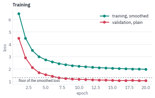
The validation loss falls fast for a few epochs and then flattens: most of what this model can learn from Tatoeba, it learns early. The training curve lies above the validation one, which looks backwards and isn’t: it is measured with label smoothing, which can’t go below the dashed floor, and with dropout switching off a tenth of the model at every step. Only the validation curve is plain cross-entropy, so the floor doesn’t apply to it, and late in the run it passes below the line.
The loss you train on and the number you judge by are different numbers. Compare like with like.
The probe sentences at a few points of the run:
shown_epochs = [1, 2, 3, 5, 10, EPOCHS]
progress = history_table[history_table.epoch.isin(shown_epochs)]
table(progress[["epoch", *PROBES]])
| epoch | The researcher said she was exhausted. | Tom forgot to lock the door. | I can't believe you did that. |
|---|---|---|---|
| 1 | С С очень очень очень | Том хотел дверь. | Я не могу это это это. |
| 2 | Корррр, что она сказала. | Том забыл, чтобы я забыл дверь. | Я не могу, что ты это сделал. |
| 3 | Старрр сказала, что она измер. | Том забыл запереть дверь. | Не могу поверить, что ты это сделал. |
| 5 | Мерник сказал, что она изможён. | Том забыл запереть дверь. | Я не могу поверить, что ты это сделал. |
| 10 | Исследование сказал, что она измощена. | Том забыл запереть дверь. | Не могу поверить, что ты это сделал. |
| 20 | Исследователи сказали, что она измотанная. | Том забыл запереть дверь. | Поверить не могу, что ты это сделал. |
In the first epoch the model strings frequent words together and repeats itself. Within a few epochs the everyday sentences come out right and stay right. Our own sentence improves too, from nonsense to nearly correct Russian, but never to the right translation: the researcher never becomes a woman. Section 10 finds out why.
8. Decoding by search
The trained model gives, for any English sentence and any Russian prefix, a probability for every possible next token. A translation needs a whole sentence, and the step from one to the other is less innocent than it looks. In training the decoder always read the correct Russian prefix; when it translates, it reads its own output, and an early mistake becomes the history every later word is written from. Here is a real case, from the translator we will compete with:
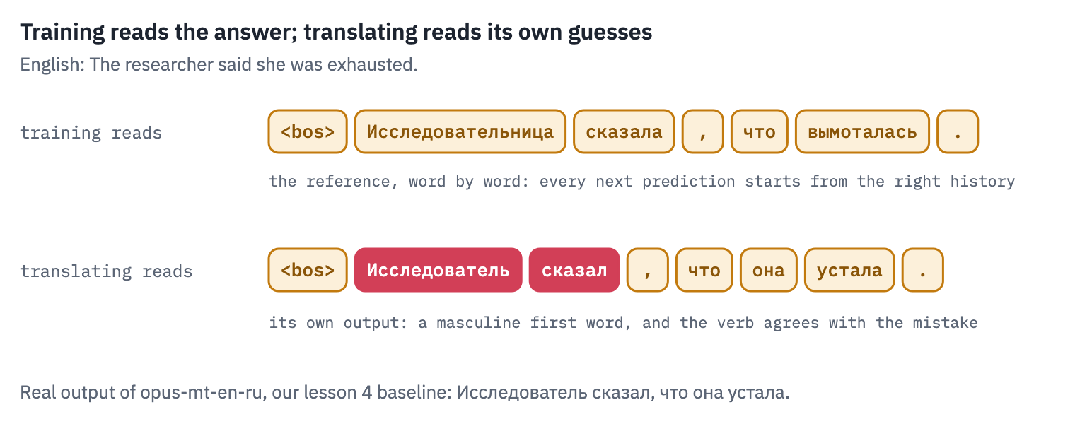
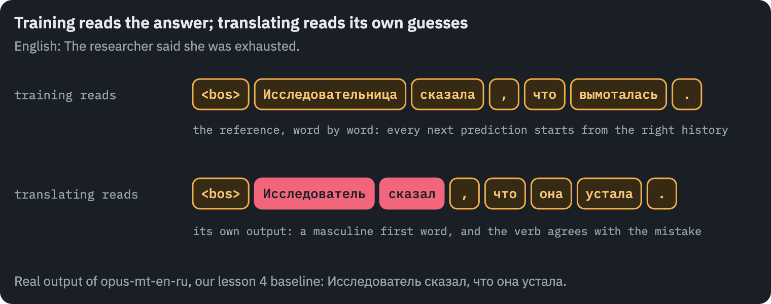
The first word came out masculine, and the verb, written after it, agrees with it. The sentence is good Russian, and it says something else: a man said that some woman was tired. The English most naturally means one person; the Russian can only mean two.
Start from the best model of the training run, and from greedy decoding, the simplest procedure: at every step take the single most probable token. Next to each translation, print its score, the log-probability the model gives the whole sentence, \(\log P(\mathbf{y} \mid \mathbf{x}) = \sum_t \log p(y_t \mid y_{<t}, \mathbf{x})\): the sum of the log-probabilities of its tokens, closer to 0 for more probable sentences.
model.load_state_dict(torch.load(CHECKPOINT, map_location=device))
model.eval()


@torch.no_grad()
def sentence_score(model, sentence, translation):
    src_ids = torch.tensor([tokenizer.encode(sentence).ids], device=device)
    ids = tokenizer.encode(translation).ids
    tgt_in = torch.tensor([[BOS] + ids], device=device)
    tgt_out = torch.tensor([ids + [EOS]], device=device)
    log_probs = model(src_ids, tgt_in).float().log_softmax(dim=-1)[0]  # (T, |V|)
    positions = torch.arange(len(ids) + 1)
    # at every position, the log-probability of the token that comes next; <eos> included
    return log_probs[positions, tgt_out[0]].sum().item()


MINIMAL_PAIRS = [
    "The researcher said she was exhausted.",
    "The researcher said he was exhausted.",
    "The teacher said she was tired.",
    "The teacher said he was tired.",
    "My neighbour said she was busy.",
    "My neighbour said he was busy.",
]

rows = []
for sentence in MINIMAL_PAIRS:
    translation = translate_greedy(model, sentence)
    score = sentence_score(model, sentence, translation)
    rows.append({"English": sentence, "greedy": translation, "score": score})
table(pd.DataFrame(rows))
| English | greedy | score |
|---|---|---|
| The researcher said she was exhausted. | Исследователи сказали, что она измотанная. | -4.40 |
| The researcher said he was exhausted. | Исследователи сказали, что он измотан. | -3.02 |
| The teacher said she was tired. | Учитель сказал, что она устала. | -0.76 |
| The teacher said he was tired. | Учитель сказал, что он устал. | -1.43 |
| My neighbour said she was busy. | Мой сосед сказал, что она занята. | -1.58 |
| My neighbour said he was busy. | Мой сосед сказал, что занят. | -1.47 |
The pronoun and the words after it follow the English: она with a feminine form for she, он or a masculine занят for he (Russian often drops the pronoun there). The first half never changes with the pronoun: the person who speaks is a man, or several people, whatever the English says. The sentences about the teacher and the neighbour, simple and frequent in the data, get scores much closer to 0 than those about the researcher, a rare word. Hold these observations until section 10.
Greedy decoding commits to every token for good. The most probable next token, though, isn’t always the start of the most probable sentence:
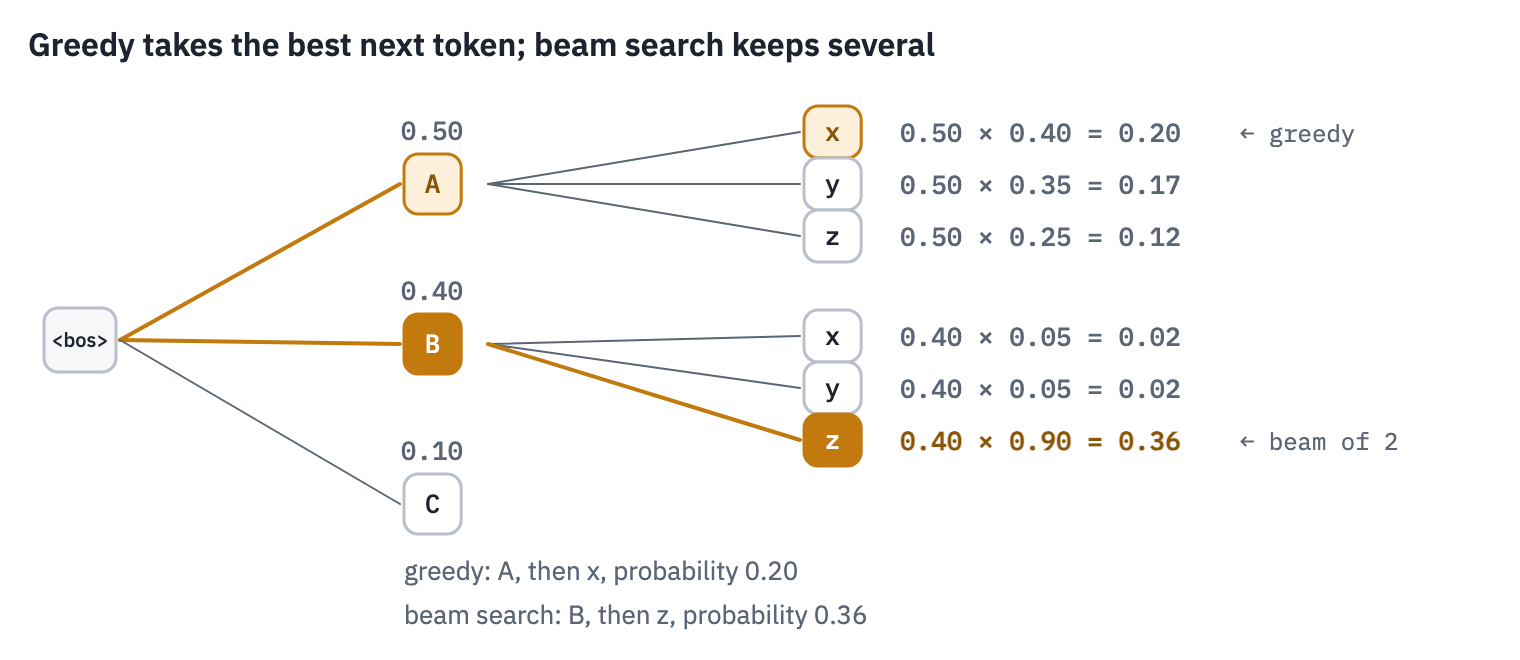
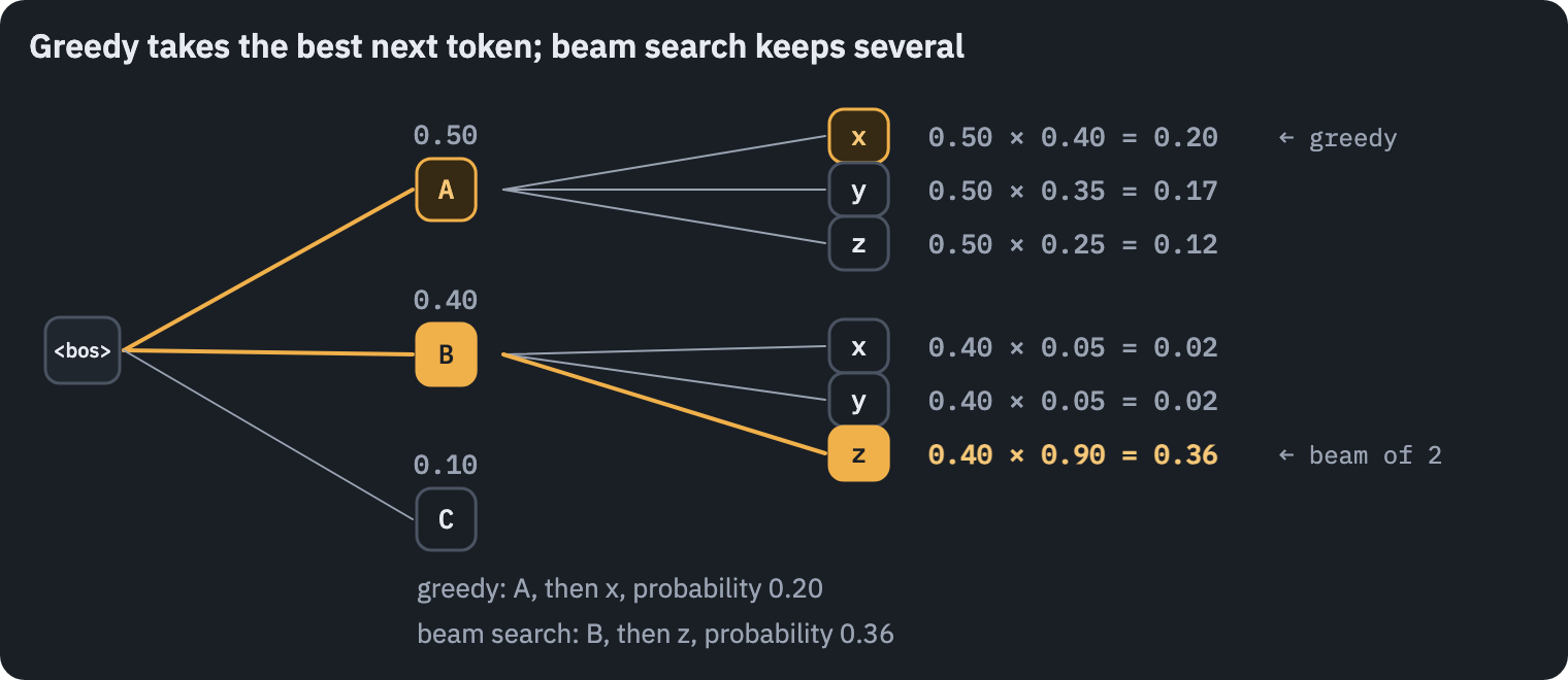
Beam search keeps the \(k\) most probable partial translations (the beam) instead of one. At every step it extends each of them by every possible token, scores all \(k \cdot \lvert\mathcal{V}\rvert\) candidates by their total log-probability, and keeps the best \(k\). A candidate that ends with <eos> is finished and set aside. With \(k = 1\) it is greedy decoding; with \(k\) as large as the number of possible sentences it would find the most probable translation exactly, at an impossible cost. In between, a handful of beams already catches most of the cases where greedy goes wrong.
One correction is needed. Every token multiplies the probability by a number below 1, so longer sentences always have lower scores, and a plain beam search prefers translations that stop early. The usual fix divides the score by a length penalty (Wu et al., 2016),
\[\operatorname{lp}(\mathbf{y}) = \left(\frac{5 + \lvert\mathbf{y}\rvert}{6}\right)^{\alpha},\]which grows with the length \(\lvert\mathbf{y}\rvert\); \(\alpha = 0\) switches it off, and the 2017 paper used \(\alpha = 0.6\) with \(k = 4\).
def length_penalty(length, alpha=0.6):
    return ((5 + length) / 6) ** alpha
The search keeps a list of beams, each a list of tokens with its total log-probability, and a list of finished translations. Every step feeds all beams to the decoder as one batch:
@torch.no_grad()
def beam_search(model, sentence, beam_size=4, alpha=0.6, max_tokens=60, trace=None):
    model.eval()
    src_ids = torch.tensor([tokenizer.encode(sentence).ids], device=device)
    memory = model.encode(src_ids)
    beams = [([BOS], 0.0)]  # (tokens so far, their total log-probability)
    finished = []

    for _ in range(max_tokens):
        k = len(beams)
        tgt = torch.tensor([tokens for tokens, _ in beams], device=device)  # one batch
        scores = model.decode(tgt, memory.expand(k, -1, -1), src_ids.expand(k, -1))[:, -1]
        log_probs = scores.float().log_softmax(dim=-1)  # (k, |V|)

        candidates = []
        for (tokens, total), row in zip(beams, log_probs):
            top = row.topk(beam_size)  # more than beam_size per beam can never survive
            for log_p, token_id in zip(top.values.tolist(), top.indices.tolist()):
                candidates.append((tokens + [token_id], total + log_p))
        candidates.sort(key=lambda candidate: candidate[1], reverse=True)  # best first

        beams = []
        for tokens, total in candidates:
            if tokens[-1] == EOS:
                finished.append((tokens, total))
            else:
                beams.append((tokens, total))
            if len(beams) == beam_size:
                break
        if trace is not None:
            trace.append([(tokenizer.decode(tokens[1:]), total) for tokens, total in beams])
        if len(finished) >= beam_size:
            break

    def normalized(candidate):
        tokens, total = candidate
        return total / length_penalty(len(tokens) - 1, alpha)  # length without <bos>

    best_tokens, _ = max(finished or beams, key=normalized)
    return tokenizer.decode(best_tokens[1:])  # decode drops <eos>
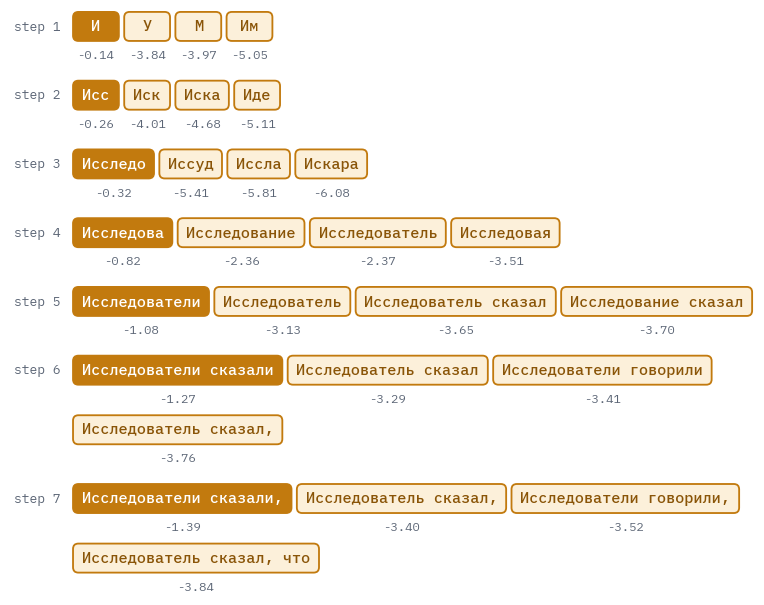
Watch the four beams grow on our sentence during the first steps, each partial translation with its total log-probability under it, the leader of every step filled.
trace = []
beam = beam_search(model, EN_EXAMPLE, trace=trace)

rows, totals, labels = [], [], []
for step in range(min(7, len(trace))):
    rows.append([text for text, _ in trace[step]])
    totals.append([f"{total:.2f}" for _, total in trace[step]])
    labels.append(f"step {step + 1}")

def is_leader(row, col, text):
    return col == 0  # the best partial translation of each step


token_chips(rows, ids=totals, labels=labels, strong=is_leader, mark_spaces=False, size=10)
plt.show()
print("greedy:     ", translate_greedy(model, EN_EXAMPLE))
print("beam search:", beam)
greedy:      Исследователи сказали, что она измотанная.
beam search: Исследователи сказали, что она измотанная.
Every step keeps four partial translations, ranked by their total log-probability, which only goes down as they grow. The runners-up are the alternatives the search weighs: a plural subject, a different verb form, sometimes a word that doesn’t exist, which falls behind and is dropped. The plural Исследователи takes the lead early and keeps it, so for this sentence beam search ends where greedy decoding does; the singular Исследователь stays in the beam as a runner-up. On other sentences an alternative overtakes the leader, as the comparison below shows.
Compare the two decoders on validation sentences: how often beam search changes the translation, and whether the translations it picks are more probable under the model, which is what it searches for.
n_sample = 150 if not SMOKE else 5
sample_pairs = valid.drop_duplicates("en").sample(n_sample, random_state=SEED)

rows = []
start = time.perf_counter()
for en, ru in zip(sample_pairs.en, sample_pairs.ru):
    greedy = translate_greedy(model, en)
    beam = beam_search(model, en)
    rows.append(
        {
            "English": en,
            "reference": ru,
            "greedy": greedy,
            "beam": beam,
            "greedy score": sentence_score(model, en, greedy),
            "beam score": sentence_score(model, en, beam),
        }
    )
decoded = pd.DataFrame(rows)
seconds = round(time.perf_counter() - start)
print("decoded", len(decoded), "sentences twice in", seconds, "s")

changed = decoded[decoded.greedy != decoded.beam]
print(f"beam search changed {len(changed)} of {len(decoded)} translations")
print("average score, greedy:", round(decoded["greedy score"].mean(), 3))
print("average score, beam:  ", round(decoded["beam score"].mean(), 3))
table(changed[["English", "reference", "greedy", "beam"]].head(6))
decoded 150 sentences twice in 14 s
beam search changed 35 of 150 translations
average score, greedy: -2.965
average score, beam: -2.551| English | reference | greedy | beam |
|---|---|---|---|
| But father, what if something happens to you? | Но, отец, а если с тобой что-то случится? | А отец, что с тобой происходит? | Но отец, что с тобой происходит? |
| Tom sang and Mary danced. | Том пел, а Мария танцевала. | Том пел, а Мэри танцевала. | Том пел и Мэри танцевали. |
| Do you have a Twitter account? | У тебя есть аккаунт в Твиттере? | У тебя есть аккаунт в Твитте? | У тебя есть аккаунт в Твиттере? |
| Tom is only bluffing. | Том всего лишь блефует. | Том всего лишь блефует. | Том лишь блефует. |
| He took off his coat and put it on again. | Он снял своё пальто и снова надел его. | Он снял пальто и снова его надел. | Он снял пальто и снова надел его. |
| We do need you. | Ты нам очень нужен. | Ты нам действительно нужен. | Вы нам действительно нужны. |
Beam search changes some of the translations, and the ones it picks score higher under the model on average, which is what it searches for. Whether they are also better translations is a separate question, sentence by sentence; lesson 4 answers it with metrics that compare outputs with the references.
9. Decoding by sampling
Search looks for the single most probable output. For a translation that’s what we want. For a chat model, or any open-ended text, it is not: the most probable continuation of a conversation is bland, and beam search on long open text famously falls into repeating itself (Holtzman et al., 2020). Those models sample instead: at every step they draw the next token at random, with the probabilities the model gives.
Two knobs shape the draw. The temperature \(\tau\) divides the scores before softmax,
\[p_j = \frac{e^{z_j / \tau}}{\sum_k e^{z_k / \tau}}:\]\(\tau < 1\) sharpens the distribution towards the most probable tokens, \(\tau > 1\) flattens it, and as \(\tau \to 0\) sampling becomes greedy decoding. Here is the distribution of the next token after Исследовательница сказала, что at three temperatures:
prefix = "Исследовательница сказала, что"
src_ids = torch.tensor([tokenizer.encode(EN_EXAMPLE).ids], device=device)
tgt = torch.tensor([[BOS] + tokenizer.encode(prefix).ids], device=device)
with torch.no_grad():
    next_scores = model(src_ids, tgt)[0, -1].float().cpu()

top_ids = next_scores.topk(8).indices.tolist()
labels = [tokenizer.id_to_token(i) for i in top_ids] + [f"the other\n{VOCAB_SIZE - 8:,}"]
fig, axes = plt.subplots(1, 3, figsize=(10, 3.2), sharey=True)
for ax, temperature in zip(axes, [0.5, 1.0, 1.5]):
    probs = (next_scores / temperature).softmax(dim=-1)
    top = probs[top_ids]
    rest = 1 - top.sum()  # all the other tokens together
    ax.bar(range(8), top, color=COLORS["data"])
    ax.bar(8, rest, color=COLORS["muted"])
    ax.set_xticks(range(9), labels, rotation=60, fontsize=9)
    ax.set_title(f"temperature {temperature}", fontsize=10)
axes[0].set_ylabel("probability")
plt.tight_layout()
plt.show()
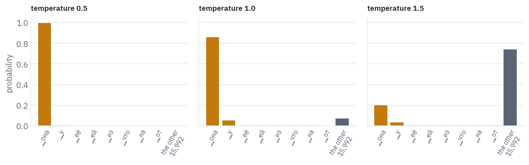
A low temperature hands almost everything to the most probable token. At temperature 1 the model’s own distribution shows a long tail: the grey bar, every token outside the top eight, together. At 1.5 that tail takes most of the probability, and a random draw will usually come from it.
The second knob, top-p or nucleus sampling, cuts off the long tail: sort the tokens by probability, keep the smallest set whose probabilities add up to at least \(p\), and sample only from that set, renormalized. The tail of thousands of individually unlikely tokens holds a surprising share of the probability in total, and a single draw from it can derail a sentence.
@torch.no_grad()
def translate_sampling(model, sentence, temperature=1.0, top_p=1.0, max_tokens=60):
    model.eval()
    src_ids = torch.tensor([tokenizer.encode(sentence).ids], device=device)
    memory = model.encode(src_ids)
    written = [BOS]
    for _ in range(max_tokens):
        tgt = torch.tensor([written], device=device)
        scores = model.decode(tgt, memory, src_ids)[0, -1].float()
        probs = (scores / temperature).softmax(dim=-1)

        if top_p < 1.0:
            sorted_probs, order = probs.sort(descending=True)
            before = sorted_probs.cumsum(dim=0) - sorted_probs  # mass of the tokens ahead
            in_nucleus = before < top_p  # keep tokens until the running total reaches top_p
            probs = torch.zeros_like(probs)
            probs[order[in_nucleus]] = sorted_probs[in_nucleus]
            probs = probs / probs.sum()

        next_id = torch.multinomial(probs, 1).item()  # one random draw
        if next_id == EOS:
            break
        written.append(next_id)
    return tokenizer.decode(written[1:])
Three draws each, at three settings: the model’s own distribution, the chat models’ setting of section 1, and a hot one.
torch.manual_seed(SEED)
rows = []
for name, settings in [
    ("temperature 1", dict(temperature=1.0)),
    ("temperature 0.6, top-p 0.9", dict(temperature=0.6, top_p=0.9)),
    ("temperature 1.5", dict(temperature=1.5)),
]:
    for _ in range(3):
        translation = translate_sampling(model, EN_EXAMPLE, **settings)
        rows.append({"settings": name, "translation": translation})
table(pd.DataFrame(rows))
| settings | translation |
|---|---|
| temperature 1 | Исследователь сказал, что она изможённа. |
| temperature 1 | Утрои Прис попробуем Откуда-то измо нарушён. |
| temperature 1 | Исследованная тяжалась передо приезжающаясь have. |
| temperature 0.6, top-p 0.9 | Исследователи сказали, что она изможена. |
| temperature 0.6, top-p 0.9 | Исследователи сказали, что она измота. |
| temperature 0.6, top-p 0.9 | Исследователи сказали, что она изможена. |
| temperature 1.5 | Ижарselvestestairs лекарства атkingthплее просить. psy.ением вегетариа stateинys согласна. неё какаяхи запас присобе носит.ерк ногтиucleри ктостьghediansсси piecesсер Р brought rescued бо but diamonduteченвидноck написано гряставили carr тупой наружу. handwrit относительно |
| temperature 1.5 | Искатка зарпла nature попросишь fish Ваши бercвания пусты studied mat.врознаваются.сь пара contain кровьжный begin узнает маме учё умный удостожденияologistбой Дождь improve странныйationоружении шкаф diary Two |
| temperature 1.5 | ваешьсяпет ЖальТы встрече cup cupранцмучен hope ровно привет попросилапечаткли напуга mu юмораум фанановый билеты заплачет сом chat шутишьейчас visitingegялась instead менееamidubeдерж great ху breadнтересоваться процерик Ещёшка подтвержд great поте M Кто asked |
At temperature 1 the samples wander: a draw from the long tail of sixteen thousand tokens now and then, and the tail includes English tokens, because lesson 1 built one vocabulary for both languages. At 1.5 the output falls apart. A low temperature with a top-p cut-off, the setting of the chat models in section 1, stays close to the greedy translation and varies a little from draw to draw. For a translation that variety is no virtue: we want the one best reading, and that’s why translators search.
10. Inside the trained model
Lesson 2 ended with a flat map: after memorizing sixteen pairs, the cross-attention of the last decoder layer spread evenly over the English sentence. Here are the same maps for the trained model, one per decoder layer, side by side, each averaged over the four heads. The model reads the reference translation of our sentence, and each row is the step at which it writes one Russian token: the row labelled ▁сказала is where the model decides on сказала, and its cells show which English tokens it looks at while doing so.
RU_EXAMPLE = "Исследовательница сказала, что вымоталась."
ru_ids = tokenizer.encode(RU_EXAMPLE).ids
src_ids = torch.tensor([tokenizer.encode(EN_EXAMPLE).ids], device=device)
tgt_in = torch.tensor([[BOS] + ru_ids], device=device)
with torch.no_grad():
    logits = model(src_ids, tgt_in)  # the attention modules keep their weights

en_tokens = tokenizer.encode(EN_EXAMPLE).tokens
written = tokenizer.encode(RU_EXAMPLE).tokens + ["<eos>"]  # row t writes token t

fig, axes = plt.subplots(1, len(model.decoder), figsize=(9, 4.6), sharey=True)
for number, (layer, ax) in enumerate(zip(model.decoder, axes), start=1):
    weights = layer.cross_attention.weights[0].mean(dim=0).float().cpu()  # (T_ru, T_en)
    title = f"decoder layer {number}"
    heatmap(weights, rows=written, cols=en_tokens, vmax=1, ax=ax, title=title)
axes[0].set_ylabel("the Russian token being written")
axes[1].set_xlabel("English (keys)")
plt.tight_layout()
plt.show()
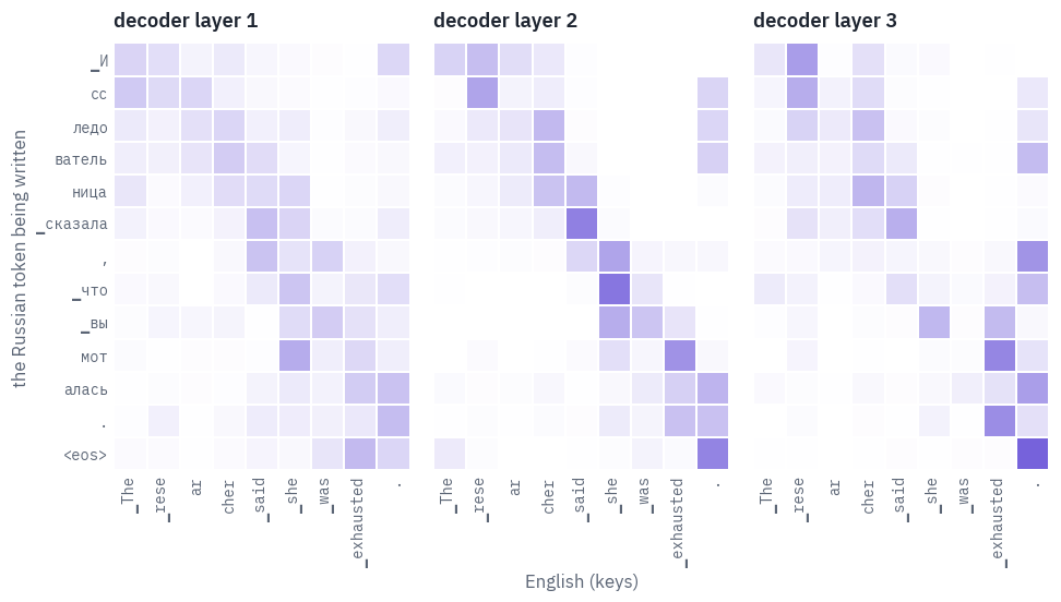
Lesson 2’s flat map is gone. For every Russian token, the English token each layer looks at most:
rows = []
for t, token in enumerate(written):
    row = {"writing": token}
    for number, layer in enumerate(model.decoder, start=1):
        weights = layer.cross_attention.weights[0].mean(dim=0)[t]  # this step, all heads
        row[f"layer {number} looks at"] = en_tokens[weights.argmax().item()]
    rows.append(row)
table(pd.DataFrame(rows))
| writing | layer 1 looks at | layer 2 looks at | layer 3 looks at |
|---|---|---|---|
| ▁И | ▁The | ▁rese | ▁rese |
| сс | ▁The | ▁rese | ▁rese |
| ледо | cher | cher | cher |
| ватель | cher | cher | . |
| ница | ▁she | ▁said | cher |
| ▁сказала | ▁said | ▁said | ▁said |
| , | ▁said | ▁she | . |
| ▁что | ▁she | ▁she | . |
| ▁вы | ▁was | ▁she | ▁she |
| мот | ▁she | ▁exhausted | ▁exhausted |
| алась | . | . | . |
| . | . | ▁exhausted | ▁exhausted |
| <eos> | ▁exhausted | . | . |
The decoder has learned an alignment: while writing the stem Исследо-ватель it looks at the pieces of researcher, while writing сказала at said, while writing -мот- at exhausted, and while writing что, the start of the clause about her, at she. Nobody told the model which word translates which. Looking at the right English word made the next token easier to predict, and training found that out on its own. The maps above show that the middle layer points most sharply; the others spread their attention more widely.
That answers the question lesson 2 left open: сказала doesn’t look at she. It doesn’t need to, as you are about to see.
So the attention works. Why, then, does the model never write Исследовательница? Ask it directly: give it the reference translation and read off the probability it assigns to each token at the moment of writing it. Tokens it finds unlikely, below 0.1, are filled:
probs = logits[0].float().softmax(dim=-1)  # (T, |V|)
targets = ru_ids + [EOS]
token_probs = [probs[t, token_id].item() for t, token_id in enumerate(targets)]

token_chips(
    [written],
    ids=[[f"{p:.2f}" for p in token_probs]],  # the probability under each token
    strong=lambda row, col, token: token_probs[col] < 0.1,
)
plt.show()

The model is sure of Исследо-, much less sure of -ватель, and gives the feminine suffix ница almost nothing. Once ница is in place (we supplied it), сказала becomes likely: agreement inside Russian, from one word to the next, the model has learned. What it hasn’t learned is to make the noun feminine because of a she that comes three words later in the English. (The other filled tokens are choices, not grammar: the model would rather continue что она than что вы-, and after the rare вымоталась it doesn’t expect the sentence to end.)
And while it writes that suffix, does it look at she at all? Every head of every layer, at that one step:
step = written.index("ница")
rows, labels = [], []
for number, layer in enumerate(model.decoder, start=1):
    for head in range(layer.cross_attention.n_heads):
        rows.append(layer.cross_attention.weights[0, head, step].float().cpu())
        labels.append(f"layer {number}, head {head + 1}")
at_suffix = torch.stack(rows)  # (layers × heads, T_en)

title = "Where each head looks while writing «ница»"
heatmap(at_suffix, rows=labels, cols=en_tokens, vmax=1, title=title)
plt.show()

she = en_tokens.index("▁she")
print("the most any head gives to ▁she here:", round(at_suffix[:, she].max().item(), 2))
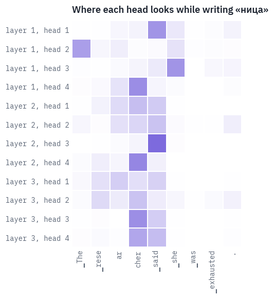
the most any head gives to ▁she here: 0.63Most heads look at said and at the end of researcher. But one head of the first layer gives most of its attention to she: the information does reach the step that decides the suffix. And still the model writes ница with a probability near zero. Looking at the right word is not enough; the layers above must also have learned what she should do to a noun, and for that they need examples.
How many examples did they get? Look at what the training data says. For a few English nouns of people, count the training pairs, and how their Russian translations render the noun: with the masculine form or the feminine one. The patterns are word stems, so that every case form counts (учителем, учительницы). Then the same counts for the pairs whose English also contains she or her:
NOUNS = {  # English noun pattern: (stem of the masculine form, stem of the feminine form)
    "teacher": ("учител", "учительниц"),
    "student": ("студент", "студентк"),
    "neighbou?r": ("сосед", "соседк"),  # British and American spelling
    "researcher": ("исследовател", "исследовательниц"),
}
mentions_she = train.en.str.contains(r"\b(?:she|her)\b", case=False)

rows = []
for noun, (masculine, feminine) in NOUNS.items():
    has_noun = train.en.str.contains(rf"\b{noun}", case=False)
    is_feminine = train.ru.str.contains(feminine, case=False)
    is_masculine = train.ru.str.contains(masculine, case=False) & ~is_feminine
    rows.append(
        {
            "English": noun.replace("ou?", "ou"),
            "pairs": int(has_noun.sum()),
            "masculine": int((has_noun & is_masculine).sum()),
            "feminine": int((has_noun & is_feminine).sum()),
            "with she/her": int((has_noun & mentions_she).sum()),
            "of them feminine": int((has_noun & mentions_she & is_feminine).sum()),
        }
    )
table(pd.DataFrame(rows))
| English | pairs | masculine | feminine | with she/her | of them feminine |
|---|---|---|---|---|---|
| teacher | 1,269 | 989 | 104 | 74 | 24 |
| student | 900 | 549 | 69 | 66 | 21 |
| neighbour | 476 | 373 | 44 | 26 | 9 |
| researcher | 8 | 7 | 0 | 0 | 0 |
The feminine forms are a small minority, and researcher, in the few pairs where it occurs at all, is never translated as a woman. Even next to she the feminine form is far from guaranteed, and for a good reason. Here are some of those pairs:
teacher_and_she = train.en.str.contains(r"\bteacher", case=False) & mentions_she
feminine_noun = train.ru.str.contains("учительниц", case=False)
masculine_noun = train.ru.str.contains("учител", case=False) & ~feminine_noun
table(train[teacher_and_she & masculine_noun].head(5))
| en | ru |
|---|---|
| The woman speaks as if she were a teacher. | Женщина говорит так, словно она учитель. |
| Ann apologized to her teacher for coming to school late. | Анна извинилась перед учителем за то, что опоздала в школу. |
| She's our teacher. | Она наш учитель. |
| My sister has made up her mind to be a teacher. | Моя сестра решила стать учителем. |
| She always writes down every word her teacher says. | Она всегда записывает каждое слово за своим учителем. |
Often she is someone else (Ann apologized to her teacher…). And when the woman is the teacher, Russian still uses the masculine noun: Она наш учитель, Моя сестра решила стать учителем. That’s ordinary Russian, where the masculine names of professions describe women too. So the data teaches the model, correctly, that учитель is the usual word, and only rarely shows it a sentence where she forces учительница and a feminine verb. For исследовательница it never shows one at all.
A model learns the distribution of its data. Rare constructions are learned last, or not at all.
That isn’t a flaw of our small model alone, as the next section shows.
11. Next to a real translator
opus-mt-en-ru, the model we will compete with in lesson 4, is on the Hub with its weights, and the transformers library runs it in a few lines with its own default decoding, four beams. Put the two models side by side on the minimal pairs, and on a few sentences from the test set that neither has trained on:
from transformers import AutoModelForSeq2SeqLM, AutoTokenizer

opus_tokenizer = AutoTokenizer.from_pretrained("Helsinki-NLP/opus-mt-en-ru")
opus = AutoModelForSeq2SeqLM.from_pretrained("Helsinki-NLP/opus-mt-en-ru").to(device).eval()


@torch.no_grad()
def translate_opus(sentences):
    batch = opus_tokenizer(list(sentences), return_tensors="pt", padding=True).to(device)
    output = opus.generate(**batch)  # its generation_config: 4 beams
    return opus_tokenizer.batch_decode(output, skip_special_tokens=True)


test_sentences = list(test.en.sample(6, random_state=SEED))
sentences = MINIMAL_PAIRS + test_sentences
rows = []
for sentence, theirs in zip(sentences, translate_opus(sentences)):
    ours = beam_search(model, sentence)
    rows.append({"English": sentence, "ours, beam of 4": ours, "opus-mt-en-ru": theirs})
table(pd.DataFrame(rows))
| English | ours, beam of 4 | opus-mt-en-ru |
|---|---|---|
| The researcher said she was exhausted. | Исследователи сказали, что она измотанная. | Исследователь сказал, что она устала. |
| The researcher said he was exhausted. | Исследователи сказали, что он измотан. | Исследователь сказал, что он устал. |
| The teacher said she was tired. | Учитель сказал, что она устала. | Учительница сказала, что она устала. |
| The teacher said he was tired. | Учитель сказал, что он устал. | Учитель сказал, что устал. |
| My neighbour said she was busy. | Мой сосед сказал, что она занята. | Моя соседка сказала, что она занята. |
| My neighbour said he was busy. | Мой сосед сказал, что занят. | Мой сосед сказал, что он занят. |
| The novel has been translated into German. | Роман был переведён на немецкий роман. | Роман был переведен на немецкий язык. |
| I wonder why you never told me about it. | Интересно, почему ты никогда мне об этом не рассказывал. | Интересно, почему ты никогда не говорил мне об этом. |
| Arguing is no way to go about it. | Спасание — не способа пойти об этом. | Спорить - это не способ. |
| Please tell me I'm right. | Пожалуйста, скажи мне, что я прав. | Пожалуйста, скажи мне, что я прав. |
| I watch TV all the time. | Я постоянно смотрю телевизор. | Я все время смотрю телевизор. |
| Tell Tom that I may be late. | Скажи Тому, что я, возможно, опоздаю. | Скажи Тому, что я, возможно, опоздаю. |
opus-mt-en-ru gets the teacher and the neighbour right, noun and verb. It was trained on OPUS, a collection of translated texts of every kind, of which Tatoeba is one small part, and has most likely seen many more sentences like these. On the researcher it fails too, Исследователь сказал: even that much data didn’t teach it this word. The architecture is the same, number for number, as lesson 2 showed; what differs is what each model has seen.
On the sentences from the test set ours is uneven for a model trained in twenty minutes: some translations match opus-mt-en-ru’s word for word, others fall apart. That’s an impression from a dozen sentences; lesson 4 replaces it with measurements on the whole test set, with BLEU, chrF and COMET, and with an analysis of where each model goes wrong.
12. Save and publish
Lesson 4 evaluates this model on the whole test set and needs its weights. We save them in the safetensors format, which stores tensors and nothing else, so loading a file can’t run code, together with a config.json that records how to rebuild the model.
from safetensors.torch import load_file, save_file

MODEL_DIR = WORK_DIR / "model"
MODEL_DIR.mkdir(exist_ok=True)
save_file(model.state_dict(), MODEL_DIR / "model.safetensors")
(MODEL_DIR / "config.json").write_text(json.dumps(CONFIG, indent=2))

reloaded = Transformer(**CONFIG).to(device)
reloaded.load_state_dict(load_file(MODEL_DIR / "model.safetensors", device=device))
assert beam_search(reloaded, EN_EXAMPLE) == beam_search(model, EN_EXAMPLE)
print("saved and reloaded:", sorted(path.name for path in MODEL_DIR.iterdir()))
saved and reloaded: ['config.json', 'model.safetensors']layers = f'{CONFIG["n_layers"]} + {CONFIG["n_layers"]} layers, {CONFIG["n_heads"]} heads'
MODEL_CARD = f"""---
license: cc-by-2.0
language: [en, ru]
tags: [translation, transformer]
datasets: [xmarva/tfs-tatoeba-en-ru]
---
# A small English→Russian Transformer, trained from scratch
Built in lesson 3 of the course "Transformers: from scratch to production":
https://github.com/xmarva/transformers-from-scratch
- the encoder-decoder Transformer of Vaswani et al. (2017) at half its base size
- {layers}, d_model {CONFIG["d_model"]}
- trained on xmarva/tfs-tatoeba-en-ru with the tokenizer xmarva/tfs-bpe-en-ru-16k
- best validation cross-entropy: {best:.3f}
The model class is `tfs.model.Transformer` from the course repository:
```python
# pip install git+https://github.com/xmarva/transformers-from-scratch
import json
from huggingface_hub import hf_hub_download
from safetensors.torch import load_file
from tfs.model import Transformer
repo = "xmarva/tfs-transformer-en-ru"
with open(hf_hub_download(repo, "config.json")) as f:
model = Transformer(**json.load(f))
model.load_state_dict(load_file(hf_hub_download(repo, "model.safetensors")))
```
Lesson 3 shows how to translate with it, greedily or with beam search.
"""
HUB_USER = os.environ.get("TFS_HUB_USER")
hf_token = env.secret("HF_TOKEN")
if HUB_USER and hf_token and not SMOKE:
api = HfApi(token=hf_token)
model_repo = f"{HUB_USER}/tfs-transformer-en-ru"
api.create_repo(model_repo, exist_ok=True)
api.upload_folder(folder_path=str(MODEL_DIR), repo_id=model_repo)
card = MODEL_CARD.encode()
api.upload_file(path_or_fileobj=card, path_in_repo="README.md", repo_id=model_repo)
print("published", model_repo)
else:
print("not publishing; lesson 4 downloads the course's copy:")
print("xmarva/tfs-transformer-en-ru")
not publishing; lesson 4 downloads the course's copy:
xmarva/tfs-transformer-en-ru
References
- Vaswani, A. et al. (2017). Attention Is All You Need. NeurIPS. The training recipe and the decoding settings.
- Szegedy, C., Vanhoucke, V., Ioffe, S., Shlens, J., Wojna, Z. (2016). Rethinking the Inception Architecture for Computer Vision. CVPR. Label smoothing.
- Müller, R., Kornblith, S., Hinton, G. (2019). When Does Label Smoothing Help?. NeurIPS.
- Kingma, D. P., Ba, J. (2015). Adam: A Method for Stochastic Optimization. ICLR.
- Liu, L. et al. (2020). On the Variance of the Adaptive Learning Rate and Beyond. ICLR. Why Adam needs a warm-up.
- Xiong, R. et al. (2020). On Layer Normalization in the Transformer Architecture. ICML. Why post-norm Transformers do.
- Pascanu, R., Mikolov, T., Bengio, Y. (2013). On the difficulty of training recurrent neural networks. ICML. Gradient clipping.
- Micikevicius, P. et al. (2018). Mixed Precision Training. ICLR.
- Wu, Y. et al. (2016). Google’s Neural Machine Translation System. The length penalty.
- Holtzman, A., Buys, J., Du, L., Forbes, M., Choi, Y. (2020). The Curious Case of Neural Text Degeneration. ICLR. Top-p sampling.
- Stanovsky, G., Smith, N. A., Zettlemoyer, L. (2019). Evaluating Gender Bias in Machine Translation. ACL.
- Tiedemann, J., Thottingal, S. (2020). OPUS-MT: Building open translation services for the World. EAMT.