- Setup
- 1. The blueprints of real models
- 2. The plan
- 3. From tokens to vectors
- 4. Attention
- 5. Why divide by \(\sqrt{d_k}\)
- 6. Masks
- 7. Several heads
- 8. Word order
- 9. The rest of a layer
- 10. The whole model
- 11. A first run, and a parrot
- 12. Can it learn?
- 13. Our code, at the size of a real model
- References
Transformers: from scratch to production · lesson 2 of 9 · all lessons · run on Kaggle · open in Colab · code on GitHub
GPT-4o, Llama 3 and DeepSeek-V3 come from different companies, learned from different data and differ in size by orders of magnitude. Open any of them and you find the same thing: one block, stacked. Here are four real models drawn to scale, next to the one you will build in this lesson:
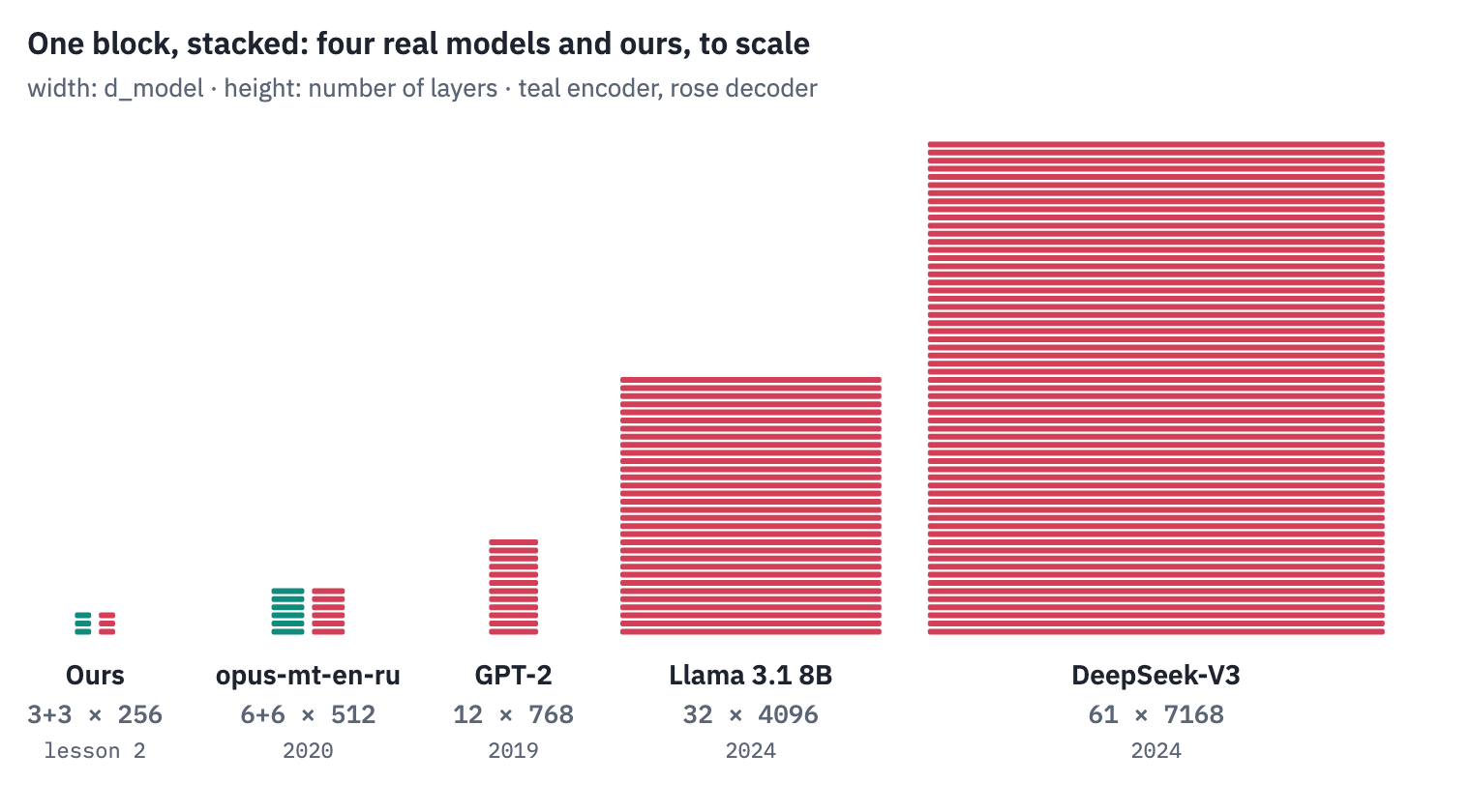
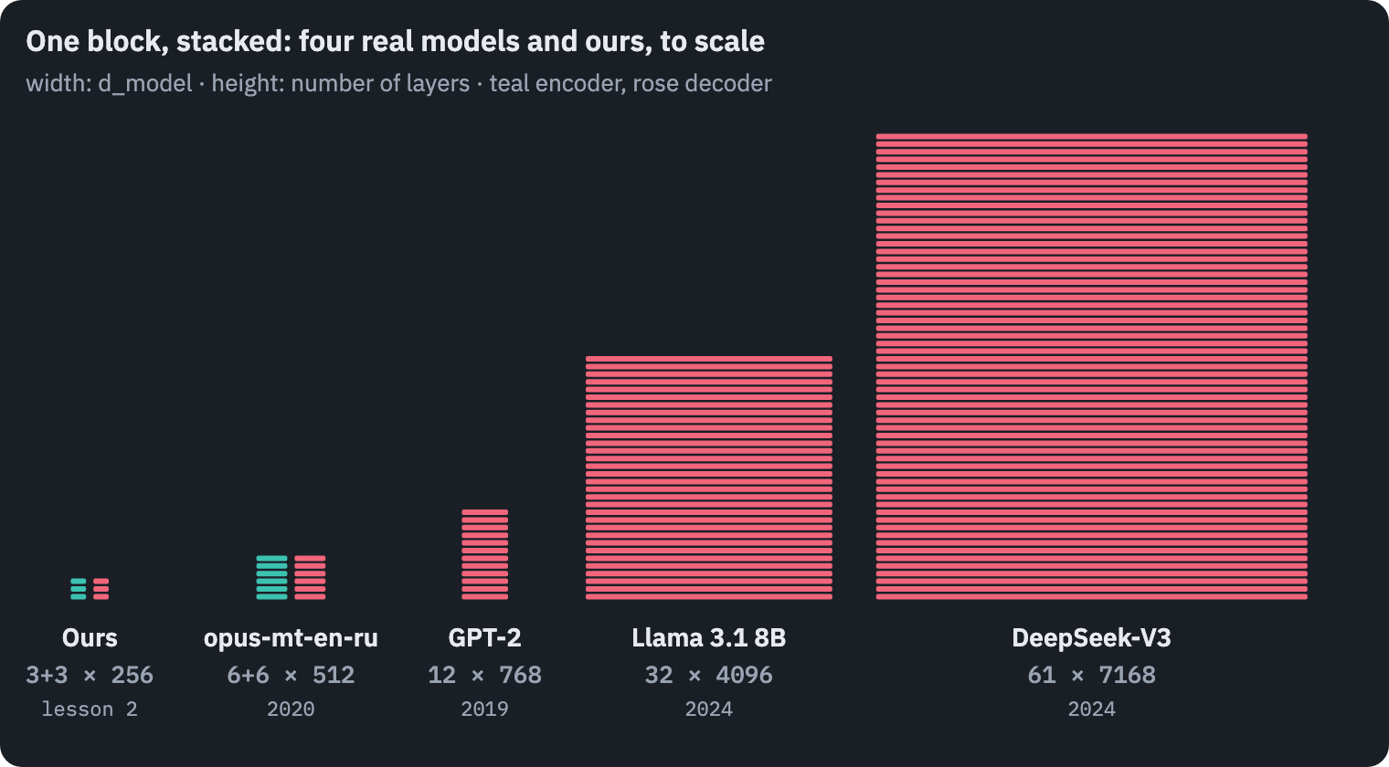
The block comes from a 2017 paper with a famous title, Attention Is All You Need (Vaswani et al.). It wasn’t about chatbots. It was about translating English into German and French, and its model, the Transformer, beat every translation system published before it. On English–German even the smaller of its two versions did, after twelve hours of training on eight GPUs.
Translation also shows best why the block is built the way it is. Take the course’s sentence:
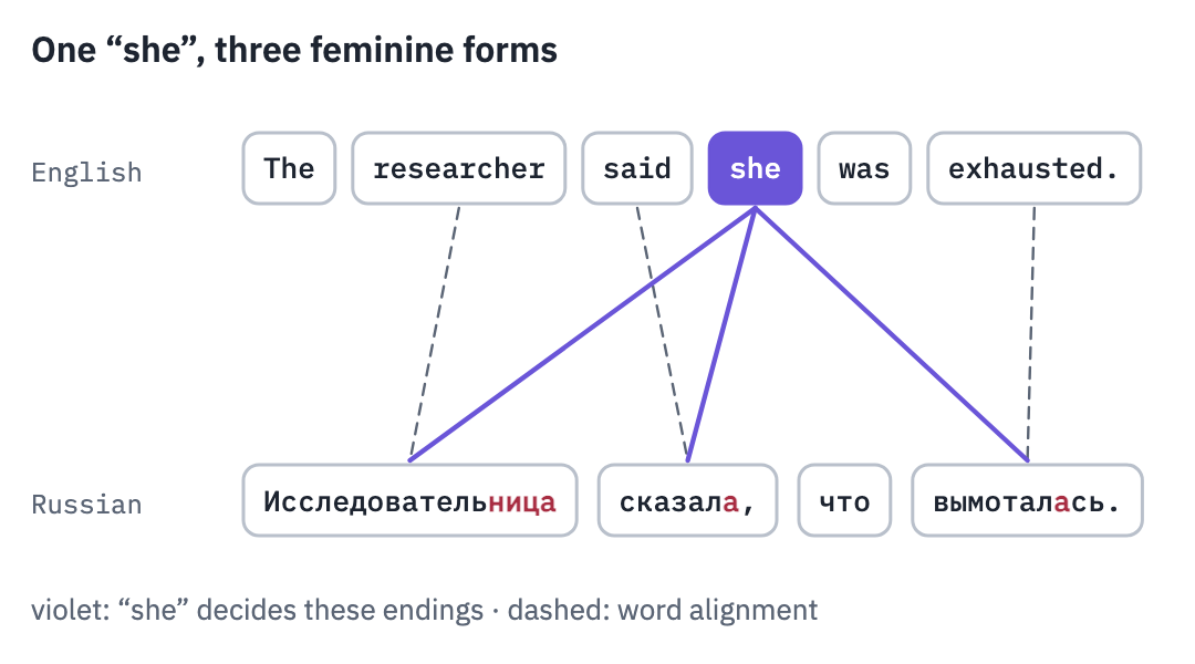
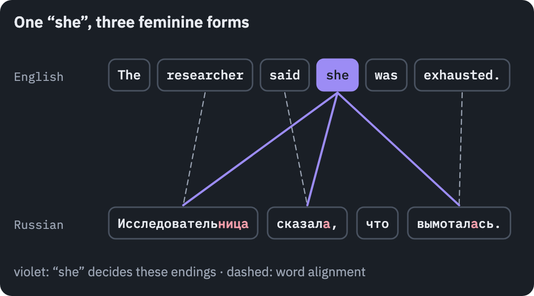
English doesn’t mark gender on researcher, said or exhausted; Russian marks it on all three. To write the very first word, Исследовательница (a woman researcher), a translator needs she, which comes later in the English sentence, and the same she decides the endings of сказала and вымоталась. The first neural translators read a sentence one word at a time and squeezed everything they might need later into a single vector of fixed size. The Transformer lets every word look directly at any other word, however far away. The mechanism is called attention, and in this lesson you build it, and the Transformer around it, line by line.
What you’ll do
- Read the blueprints of real models: GPT-2, Llama 3, DeepSeek-V3, and opus-mt-en-ru, the translator we will compete with in lesson 4.
- Build attention from its formula, see why it divides by \(\sqrt{d_k}\), and check it against PyTorch’s own.
- Add what turns attention into a Transformer: masks, several heads, word order, feed-forward layers, residual connections and normalization.
- Assemble the encoder–decoder model of the 2017 paper and test it: its loss before training matches a formula (once you see what the model is doing), and it can learn a batch of sentences by heart.
What you need: the tokenizer and the data of lesson 1, which the notebook downloads. Some PyTorch helps (tensors, nn.Module), but every step is explained. A CPU is enough; the notebook runs in a few minutes.
Setup
One small helper package, tfs, draws the course’s plots and token chips and knows where the notebook runs (Kaggle, Colab or your own machine). Everything the lesson teaches is written out in the notebook itself.
import importlib.util
import subprocess
import sys

TFS = "git+https://github.com/xmarva/transformers-from-scratch@main"
if importlib.util.find_spec("tfs") is None:
    subprocess.check_call([sys.executable, "-m", "pip", "install", "-q", TFS])

from tfs import env
from tfs.viz import table, token_chips, use_course_style

env.quiet()  # no progress bars or environment warnings in the outputs
SEED = 42
env.seed_everything(SEED)
COLORS = use_course_style()
WORK_DIR = env.work_dir()
import collections
import json
import math
import time

import matplotlib.pyplot as plt
import numpy as np
import pandas as pd
import torch
import torch.nn as nn
import torch.nn.functional as F
from huggingface_hub import HfApi, hf_hub_download
from tfs.viz import bars, heatmap
from tokenizers import Tokenizer

device = "cuda" if torch.cuda.is_available() else "cpu"
print("device:", device)
device: cpuLesson 1 published its tokenizer and its splits of the data on the Hugging Face Hub. We need the tokenizer and, for a few experiments, the validation sentences:
tokenizer_path = hf_hub_download("xmarva/tfs-bpe-en-ru-16k", "tokenizer.json")
tokenizer = Tokenizer.from_file(tokenizer_path)

valid_path = hf_hub_download(
    "xmarva/tfs-tatoeba-en-ru", "data/validation.parquet", repo_type="dataset"
)
valid = pd.read_parquet(valid_path)

VOCAB_SIZE = tokenizer.get_vocab_size()
PAD = tokenizer.token_to_id("<pad>")
BOS = tokenizer.token_to_id("<bos>")
EOS = tokenizer.token_to_id("<eos>")
print("vocabulary:", VOCAB_SIZE, "validation pairs:", len(valid))
vocabulary: 16000 validation pairs: 103701. The blueprints of real models
Every model on the Hub comes with a config.json: a few hundred bytes that describe its shape, so that a library can build the right network before loading the weights into it. Download four of them:
BLUEPRINTS = {
    "GPT-2 (2019)": "openai-community/gpt2",
    "opus-mt-en-ru (2020)": "Helsinki-NLP/opus-mt-en-ru",
    "Llama 3.1 8B (2024)": "unsloth/Meta-Llama-3.1-8B",
    "DeepSeek-V3 (2024)": "deepseek-ai/DeepSeek-V3",
}

configs = {}
for name, repo in BLUEPRINTS.items():
    with open(hf_hub_download(repo, "config.json")) as f:
        configs[name] = json.load(f)

gpt2_config = configs["GPT-2 (2019)"]
for key in ["n_layer", "n_embd", "n_head", "vocab_size", "n_positions"]:
    print(key, "=", gpt2_config[key])
n_layer = 12
n_embd = 768
n_head = 12
vocab_size = 50257
n_positions = 1024
Every lab names things its own way: GPT-2’s n_embd is Llama’s hidden_size and Marian’s d_model. (Marian is the translation toolkit behind opus-mt-en-ru.) Two small functions bring them to one table in the course’s notation: row makes one line of the table, and blueprint finds each number in a config, whatever its name there.
def row(model, layers, d_model, heads, d_ff, vocabulary, note=""):
    return {
        "model": model,
        "layers": layers,
        "d_model": d_model,
        "heads": heads,
        "d_ff": d_ff,
        "vocabulary": vocabulary,
        "note": note,
    }


def first_key(config, keys):
    for key in keys:
        if config.get(key) is not None:
            return config[key]
    return None


def blueprint(name, config):
    d_model = first_key(config, ["hidden_size", "d_model", "n_embd"])
    heads = first_key(config, ["num_attention_heads", "encoder_attention_heads", "n_head"])

    if "encoder_layers" in config:  # an encoder-decoder model has two stacks
        layers = f'{config["encoder_layers"]} + {config["decoder_layers"]}'
    else:
        layers = str(first_key(config, ["num_hidden_layers", "n_layer"]))

    d_ff = first_key(config, ["intermediate_size", "encoder_ffn_dim", "n_inner"])
    if d_ff is None:
        d_ff = 4 * d_model  # GPT-2 leaves it out; its default is four times d_model

    note = ""
    if "n_routed_experts" in config:
        n_experts, used = config["n_routed_experts"], config["num_experts_per_tok"]
        note = f"{n_experts} experts, {used} used per token"

    return row(name, layers, d_model, heads, d_ff, config["vocab_size"], note)
Our model gets its own row. Its settings live here, next to the table that compares them; D_MODEL is the width that lesson 1 used to price the embedding table. The first row is the base model of the 2017 paper, copied from its Table 3.
D_MODEL = 256
N_HEADS = 4
D_FF = 1024
N_LAYERS = 3  # in the encoder, and as many in the decoder
DROPOUT = 0.1

rows = [row("Transformer, base (2017)", "6 + 6", 512, 8, 2048, 37_000, "from the paper")]
for name, config in configs.items():
    rows.append(blueprint(name, config))
ours = f"{N_LAYERS} + {N_LAYERS}"
rows.append(row("Ours (this lesson)", ours, D_MODEL, N_HEADS, D_FF, VOCAB_SIZE))

table(pd.DataFrame(rows))
| model | layers | d_model | heads | d_ff | vocabulary | note |
|---|---|---|---|---|---|---|
| Transformer, base (2017) | 6 + 6 | 512 | 8 | 2,048 | 37,000 | from the paper |
| GPT-2 (2019) | 12 | 768 | 12 | 3,072 | 50,257 | |
| opus-mt-en-ru (2020) | 6 + 6 | 512 | 8 | 2,048 | 62,518 | |
| Llama 3.1 8B (2024) | 32 | 4,096 | 32 | 14,336 | 128,256 | |
| DeepSeek-V3 (2024) | 61 | 7,168 | 128 | 18,432 | 129,280 | 256 experts, 8 used per token |
| Ours (this lesson) | 3 + 3 | 256 | 4 | 1,024 | 16,000 |
Read the table column by column.
- layers: how many blocks are stacked. The translators (the 2017 model, opus-mt-en-ru and ours) have two stacks: an encoder that reads the source sentence and a decoder that writes the translation. GPT-2, Llama and DeepSeek keep only the decoder: they continue a text rather than translate one.
- d_model: the length of the vector that represents every token on its way through the model.
- heads and d_ff: the number of attention heads and the width of the feed-forward layer, both explained below.
- note: DeepSeek-V3 replaces most feed-forward layers with a mixture of experts, many feed-forward layers of which every token uses only a few. Changes of this kind are the subject of lesson 5; the skeleton stays the same.
Compare two rows. opus-mt-en-ru, the model we will try to beat, has exactly the shape of the 2017 base model: three years of progress in translation changed the data and the training, not the blueprint. Ours is that blueprint at half the size in every dimension, small enough to train on a free GPU in lesson 3.
2. The plan
Here is the whole model. Don’t try to read every box yet; the rest of the lesson builds them one at a time, from the bottom up, and comes back to this picture at the end.
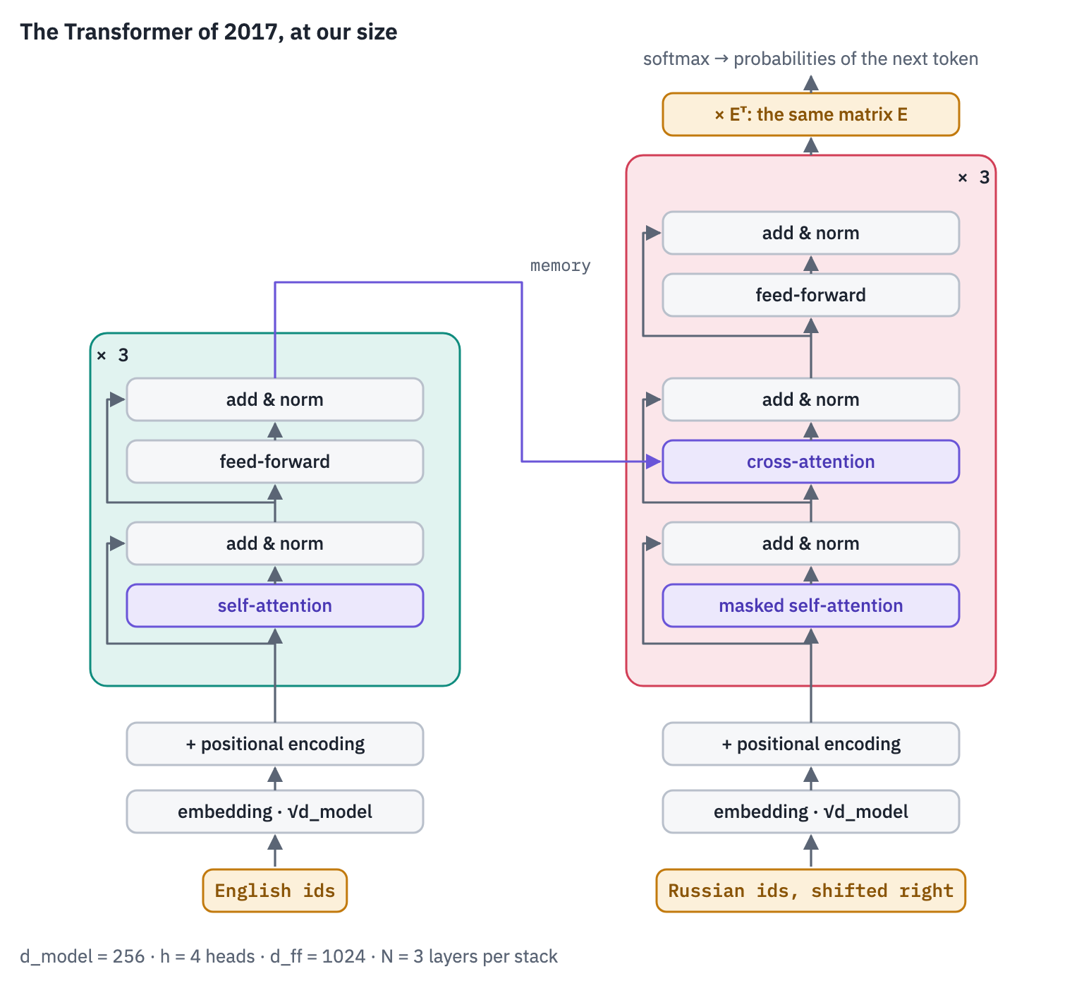
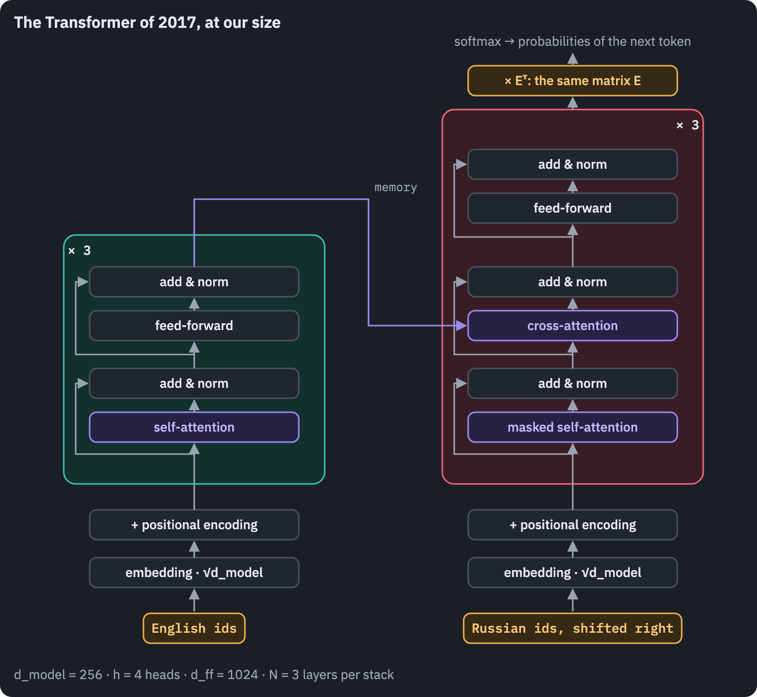
The encoder (teal) reads the English sentence. Every token becomes a vector, receives a signal about its position, and goes through \(N\) layers of two parts: self-attention, where the tokens look at each other, and a feed-forward network, which processes every token on its own. The decoder (rose) writes the Russian sentence one token at a time. Its layers have one more part, cross-attention, through which it reads the encoder’s output, called the memory. At the top, the same embedding matrix that turned tokens into vectors turns vectors back into a score for every token of the vocabulary; the highest score is the model’s guess for the next token.
3. From tokens to vectors
A model can’t do arithmetic with token ids: id 5 000 isn’t “bigger” than id 50 in any meaningful way, and ids that are neighbours aren’t related. So every token gets a vector of D_MODEL numbers instead, a row of the embedding matrix \(E \in \mathbb{R}^{\lvert\mathcal{V}\rvert \times d_{\text{model}}}\), one row per token of the vocabulary. The rows start out random. Training moves them, and tokens that are used in similar ways end up with similar vectors. That is how a model can come to treat сказал and сказала as relatives, although to it they are just two different ids.
Our sentence as token ids, the row numbers in \(E\):
EN_EXAMPLE = "The researcher said she was exhausted."
RU_EXAMPLE = "Исследовательница сказала, что вымоталась."

encoding = tokenizer.encode(EN_EXAMPLE)
src_ids = torch.tensor([encoding.ids])  # a batch of one sentence: shape (1, T)
token_chips([encoding.tokens], ids=[encoding.ids])
plt.show()

nn.Embedding stores \(E\) and looks rows up. Looking up a row is the same as multiplying a one-hot vector (all zeros except a 1 at the token’s id) by \(E\), which is why an embedding can be trained like any other layer. Rather than believe it, check it:
embedding = nn.Embedding(VOCAB_SIZE, D_MODEL)
nn.init.normal_(embedding.weight, mean=0.0, std=D_MODEL**-0.5)

vectors = embedding(src_ids)
print("vectors:", tuple(vectors.shape))  # (B, T, d_model): one vector per token

one_hot = F.one_hot(src_ids, VOCAB_SIZE).float()  # (1, T, |V|)
assert torch.allclose(one_hot @ embedding.weight, vectors)
print("looking up rows = multiplying by one-hot vectors")
vectors: (1, 9, 256)
looking up rows = multiplying by one-hot vectors
Notice the initialization: random numbers with standard deviation \(d_{\text{model}}^{-1/2}\), not PyTorch’s default. The reason is at the top of the architecture. The paper uses the same matrix \(E\) twice: as the embedding at the bottom and as the output layer at the top, where the score of token \(j\) is the dot product of the decoder’s final vector \(\mathbf{h}\) with row \(\mathbf{e}_j\):
\[z_j = \mathbf{h} \cdot \mathbf{e}_j = \sum_{i=1}^{d_{\text{model}}} h_i\, e_{ji}.\]The final vector has \(d_{\text{model}}\) entries of size about 1. A sum of \(d_{\text{model}}\) random terms, each with variance \(1/d_{\text{model}}\), has variance about 1, so the scores start out small and similar: a model that knows nothing should be unsure of everything. Section 11 tests this prediction and finds a surprise.
At the bottom, the same small rows meet the position signals of section 8, whose entries go up to 1. The position would drown out the meaning, so the paper multiplies the embeddings by \(\sqrt{d_{\text{model}}}\):
entries = vectors.flatten().detach()  # every number of the sentence's 9 vectors
scaled = entries * math.sqrt(D_MODEL)

bins = np.linspace(-4, 4, 81)
fig, axes = plt.subplots(2, 1, figsize=(6.4, 3.8), sharex=True)
axes[0].hist(entries, bins=bins, color=COLORS["data"])
axes[0].set_title("Rows of E as initialized", fontsize=10)
axes[1].hist(scaled, bins=bins, color=COLORS["data"])
axes[1].axvspan(-1, 1, color=COLORS["att"], alpha=0.12)  # where position signals live
axes[1].set_title("Times √d_model: the size of the position signals (violet)", fontsize=10)
axes[1].set_xlabel("value of an entry")
plt.tight_layout()
plt.show()

print("std of the entries:", round(entries.std().item(), 3))
print("after scaling:     ", round(scaled.std().item(), 3))
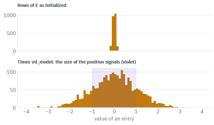
std of the entries: 0.064
after scaling:      1.024
4. Attention
Attention is a soft version of looking something up. A Python dictionary compares a query with its keys, finds the one that matches exactly and returns that key’s value. Attention compares a query with every key, gives each one a weight according to how well it matches, and returns a weighted mix of all the values:
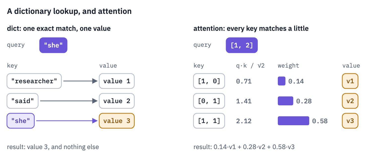
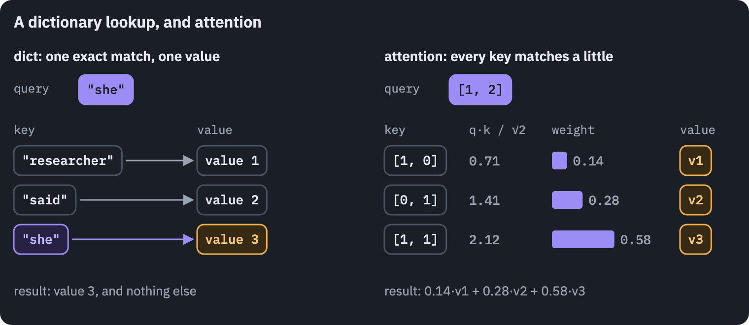
Softness is what makes it learnable. A dictionary either finds the key or doesn’t, and there is nothing to adjust in between. Attention’s weights change smoothly when the vectors change a little, so training can nudge every query, key and value in the direction that improves the translation.
In a Transformer, every token plays all three parts at once. Its vector is multiplied by three learned matrices, which gives it a query (what it is looking for), a key (how it can be found) and a value (what it hands over to those who find it):
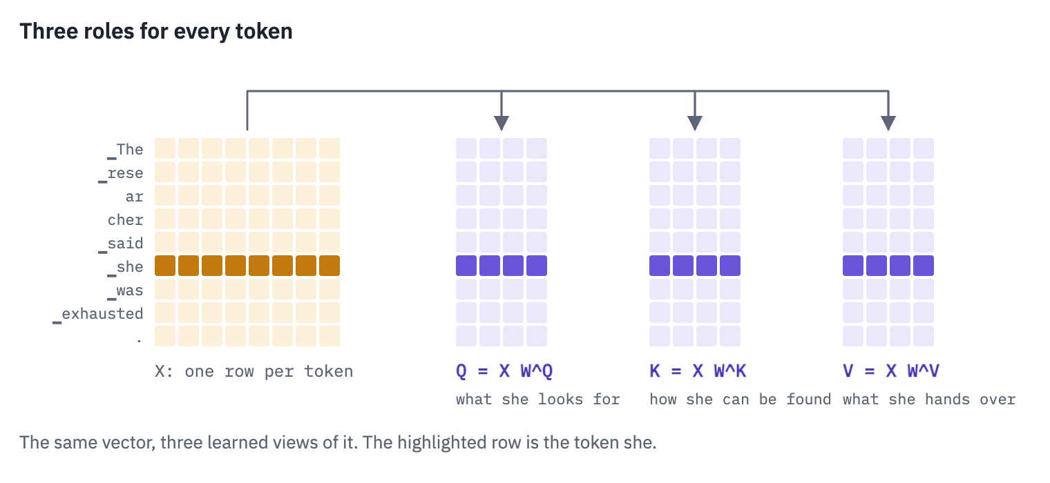
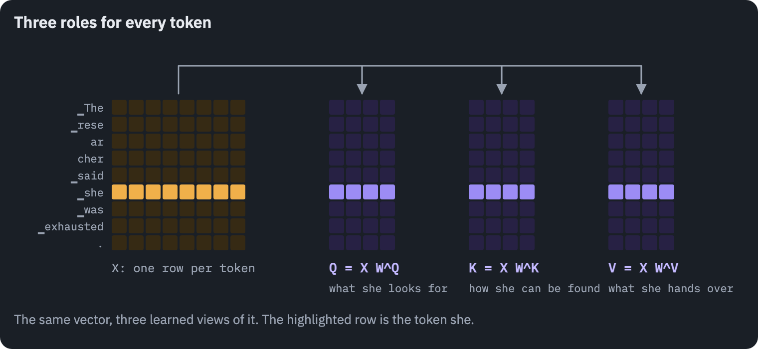
Why three separate vectors and not one? Because the roles differ. What сказала needs (the subject, its gender) is not what it offers to others (a verb in the past tense), and neither is what it passes on. Separate learned matrices let the model shape each role on its own.
The computation itself, step by step:
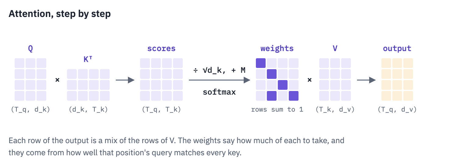
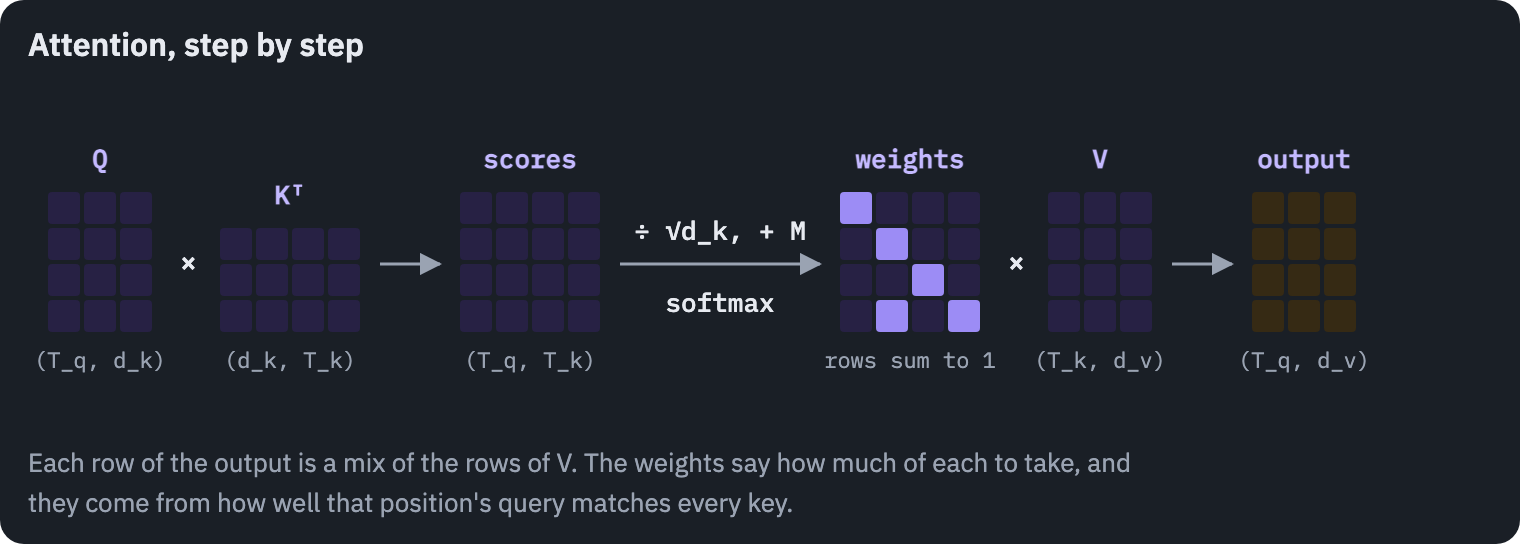
In the notation of the course, with every query, key and value as a row of a matrix:
\[\operatorname{Attention}(Q, K, V) = \operatorname{softmax}\!\left(\frac{Q K^\top}{\sqrt{d_k}} + M\right) V\]- \(Q\), shape \((T_q, d_k)\): one query per position that asks.
- \(K\), shape \((T_k, d_k)\), and \(V\), shape \((T_k, d_v)\): one key and one value per position that can be found.
- \(Q K^\top\), shape \((T_q, T_k)\): the dot product of every query with every key, all at once. A large dot product means the two vectors point the same way: a good match.
- \(\sqrt{d_k}\) keeps the scores in a range where softmax still works well; section 5 shows why.
- \(M\), the mask: \(0\) where looking is allowed and \(-\infty\) where it isn’t (section 6).
- \(\operatorname{softmax}\), applied to every row, turns scores into weights: it exponentiates them, which makes them positive and stretches the differences, and divides by their sum, so every row adds up to 1: \(\operatorname{softmax}(\mathbf{s})_i = e^{s_i} / \sum_j e^{s_j}\).
- The result, shape \((T_q, d_v)\): for every query, a weighted average of the values.
Start with the numbers of the picture above, small enough to check by hand: one query, three keys, and values that are one-hot, so that the output shows the weights themselves.
q = torch.tensor([[1.0, 2.0]])  # one query, d_k = 2
k = torch.tensor([[1.0, 0.0], [0.0, 1.0], [1.0, 1.0]])  # three keys
v = torch.eye(3)  # three one-hot values

scores = q @ k.T / math.sqrt(2)
weights = scores.softmax(dim=-1)
print("scores: ", scores)
print("weights:", weights)
print("output: ", weights @ v)
scores:  tensor([[0.7071, 1.4142, 2.1213]])
weights: tensor([[0.1400, 0.2840, 0.5760]])
output:  tensor([[0.1400, 0.2840, 0.5760]])
The dot products are \(1\), \(2\) and \(3\); divided by \(\sqrt 2\) they become the scores, and softmax turns those into weights that sum to 1. The third key matches the query best and gets the largest share, but not all of it.
Attention mixes; it doesn’t pick.
The general function is the formula, line for line. Its inputs can have any number of leading dimensions (a batch of sentences, several heads); the last two are always positions and vector entries, which is why the transpose swaps exactly those two, -2 and -1.
def attention(q, k, v, mask=None):
    d_k = q.shape[-1]
    scores = q @ k.transpose(-2, -1) / math.sqrt(d_k)  # (..., T_q, T_k): all pairs at once
    if mask is not None:
        scores = scores + mask  # -inf where looking is forbidden
    weights = scores.softmax(dim=-1)  # each row sums to 1
    return weights @ v, weights  # (..., T_q, d_v), and the weights for plotting
PyTorch has its own implementation, F.scaled_dot_product_attention, which is faster and saves memory (lesson 5 switches to it). It computes the same thing. Compare the two on random tensors of a realistic shape, with a mask that hides some positions:
q = torch.randn(2, 4, 7, 64)  # (batch, heads, positions, d_k)
k = torch.randn(2, 4, 7, 64)
v = torch.randn(2, 4, 7, 64)
mask = torch.zeros(7, 7)
mask[:, 5:] = float("-inf")  # nobody may look at the last two positions

ours, _ = attention(q, k, v, mask)
theirs = F.scaled_dot_product_attention(q, k, v, attn_mask=mask)
assert torch.allclose(ours, theirs, atol=1e-5)
print("same output as torch's scaled_dot_product_attention")
same output as torch's scaled_dot_product_attentionThe same function does two different jobs in the Transformer, depending on where the queries, keys and values come from.
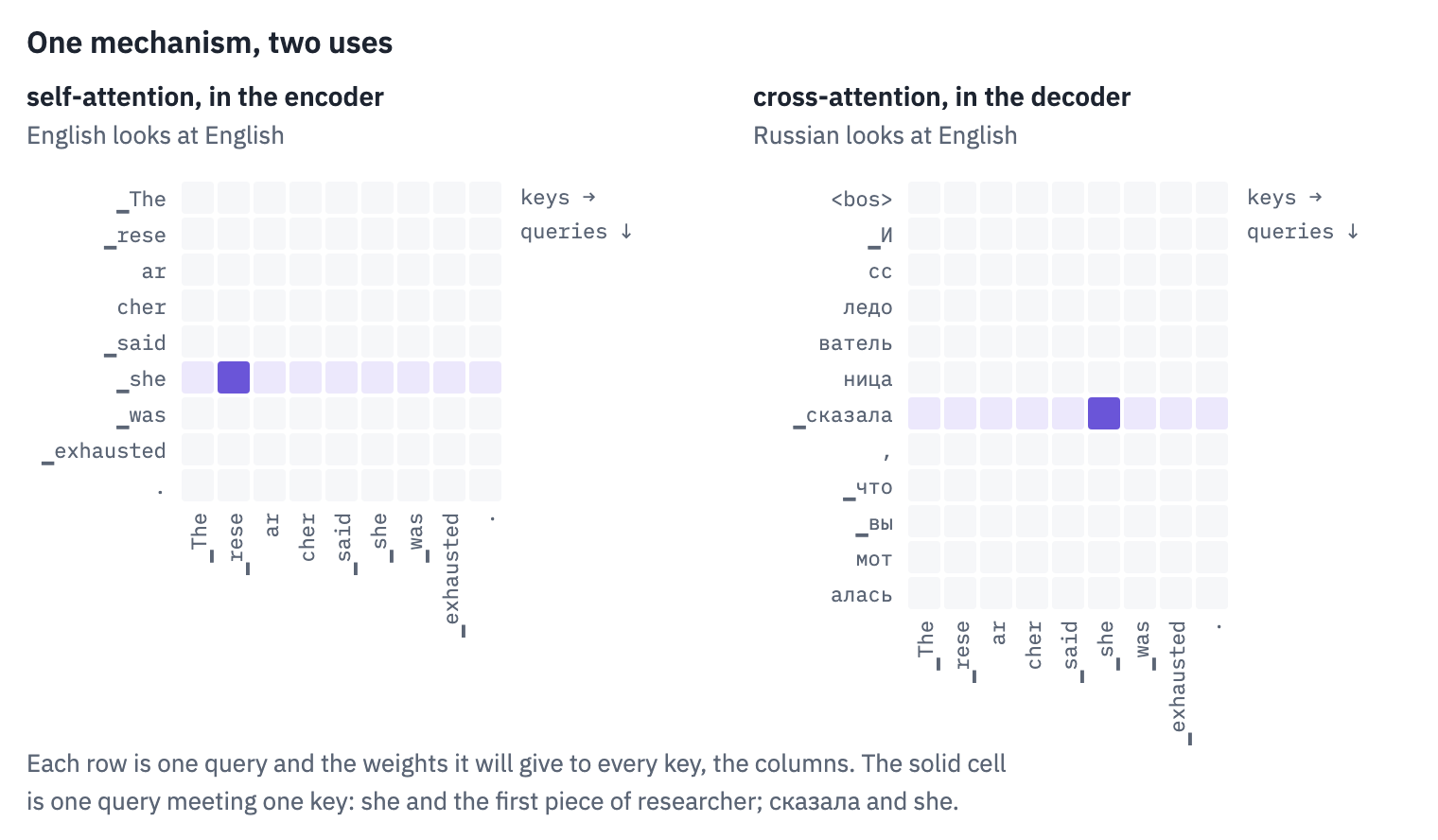
In self-attention all three come from one sentence: every English token looks at every English token, and the result is a version of the sentence in which each token knows something about its neighbours, near and far. In cross-attention the queries come from the Russian side and the keys and values from the English side: this is where the translation reads the source. The decoder also has a self-attention of its own, over the Russian tokens written so far; section 6 shows what it must not see.
5. Why divide by \(\sqrt{d_k}\)
Suppose the entries of a query \(\mathbf{q}\) and a key \(\mathbf{k}\) are independent, with mean 0 and variance 1. (A real model’s are only roughly like that, but the argument is about how things grow with \(d_k\).) Their dot product is a sum of \(d_k\) independent terms, and the variances of independent terms add up:
\[\operatorname{Var}(\mathbf{q} \cdot \mathbf{k}) = \sum_{i=1}^{d_k} \operatorname{Var}(q_i k_i) = \sum_{i=1}^{d_k} \mathbb{E}[q_i^2]\,\mathbb{E}[k_i^2] = d_k.\]So the scores spread out like \(\sqrt{d_k}\): wider heads, larger scores. Softmax exponentiates, so larger scores mean a more extreme result: almost all the weight goes to one key. That stalls learning, because the derivative of the softmax output \(p_i\) with respect to a score \(s_j\) is
\[\frac{\partial p_i}{\partial s_j} = p_i\,(\delta_{ij} - p_j),\]where \(\delta_{ij}\) is 1 when \(i = j\) and 0 otherwise. When one \(p\) is close to 1 and the rest close to 0, every one of these terms is close to 0: the scores stop receiving gradient, and the queries and keys stop learning. Dividing by \(\sqrt{d_k}\) brings the variance back to 1, whatever the width of a head.
Test both claims. For five widths of a head, take 2 000 random queries with 16 random keys each, measure the variance of the scores, and look at the weights softmax gives the keys, with and without the division. Sorting each query’s 16 weights from largest to smallest and averaging over the queries shows the typical shape:
def sorted_weights(scores):
    weights = scores.softmax(dim=-1)  # (queries, 16)
    largest_first = weights.sort(dim=-1, descending=True).values
    return largest_first.mean(dim=0)  # the typical shape over all queries


results = {}
for d_k in [4, 16, 64, 256, 1024]:
    q = torch.randn(2_000, 1, d_k)  # 2 000 random queries
    k = torch.randn(2_000, 16, d_k)  # 16 random keys for each
    scores = (q @ k.transpose(-2, -1)).squeeze(1)  # (2 000, 16)
    results[d_k] = {
        "variance": scores.var().item(),
        "raw": sorted_weights(scores),
        "scaled": sorted_weights(scores / math.sqrt(d_k)),
    }

fig, axes = plt.subplots(2, 3, figsize=(9, 4.2), sharey=True)
for col, d_k in enumerate([4, 64, 1024]):
    for row_index, version in enumerate(["raw", "scaled"]):
        ax = axes[row_index, col]
        ax.bar(range(16), results[d_k][version], color=COLORS["att"])
        ax.set_xticks([])
        label = "raw" if version == "raw" else "÷ √d_k"
        ax.set_title(f"d_k = {d_k}, {label}", fontsize=10)
axes[0, 0].set_ylabel("weight")
axes[1, 0].set_ylabel("weight")
plt.tight_layout()
plt.show()
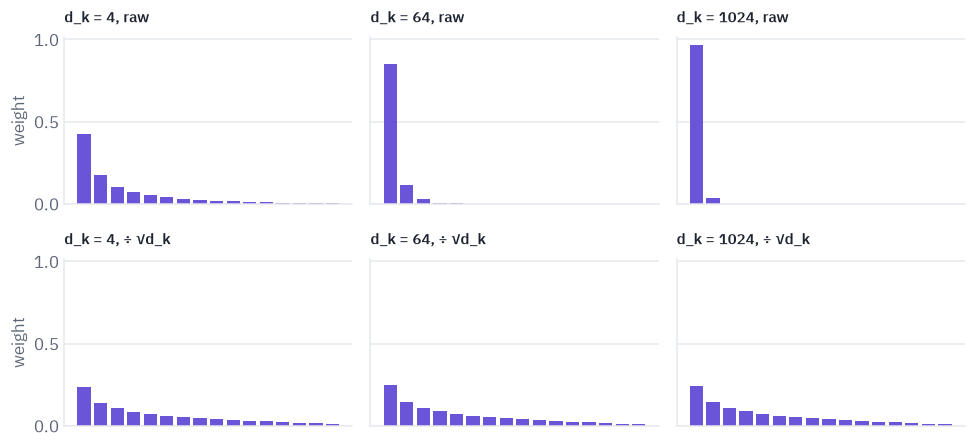
Without the division (top row), the wider the head, the more the largest score takes everything, until attention turns into a hard choice. With it (bottom row), the weights keep the same shape at every width. In numbers:
rows = []
for d_k, result in results.items():
    rows.append(
        {
            "d_k": d_k,
            "variance of q·k": result["variance"],
            "top weight, raw": result["raw"][0].item(),
            "top weight, ÷ √d_k": result["scaled"][0].item(),
        }
    )
table(pd.DataFrame(rows))
| d_k | variance of q·k | top weight, raw | top weight, ÷ √d_k |
|---|---|---|---|
| 4 | 3.96 | 0.43 | 0.23 |
| 16 | 16.35 | 0.69 | 0.25 |
| 64 | 63.05 | 0.85 | 0.25 |
| 256 | 253.85 | 0.92 | 0.24 |
| 1,024 | 998.28 | 0.96 | 0.24 |
The variance follows \(d_k\), as derived, and only the scaled weights stay put. Our heads have \(d_k = 64\), the same as in the 2017 paper.
6. Masks
Attention lets every position look at every other. Two kinds of looking must be forbidden.
Padding. Sentences in a batch have different lengths, and a tensor must be rectangular, so shorter sentences are filled up with the <pad> token. Padding isn’t part of the text, and nobody should attend to it. Make a batch of three sentences of different lengths:
def pad_batch(sequences):
    longest = max(len(ids) for ids in sequences)
    batch = torch.full((len(sequences), longest), PAD)  # start with all <pad>
    for row_index, ids in enumerate(sequences):
        batch[row_index, : len(ids)] = torch.tensor(ids)  # then each sentence from the left
    return batch


word_counts = valid.en.str.split().str.len()
short_sentence = valid.en[word_counts == 2].iloc[0]
long_sentence = valid.en[word_counts == 10].iloc[0]
sentences = [EN_EXAMPLE, short_sentence, long_sentence]

src = pad_batch([tokenizer.encode(sentence).ids for sentence in sentences])
for ids in src.tolist():
    print(ids)  # the ids the model receives; <pad> is 0
[385, 9581, 310, 15272, 683, 713, 378, 10890, 17, 0, 0]
[256, 10, 78, 10890, 17, 0, 0, 0, 0, 0, 0]
[402, 496, 462, 1157, 1894, 265, 389, 4293, 879, 1995, 17]
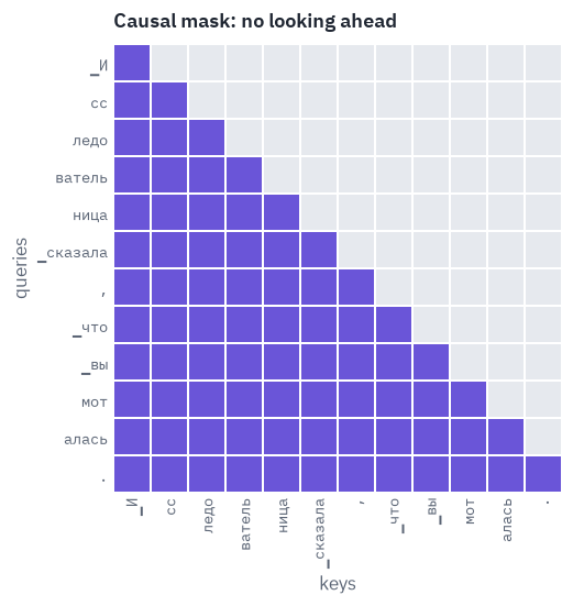
The future. The decoder is trained on whole Russian sentences at once (section 10 shows how), but when it translates, it writes one token at a time and can’t see the tokens it hasn’t written yet. So during training, position \(t\) may look only at positions up to \(t\); otherwise the model would learn to copy the next word instead of predicting it.
Both rules are written into the mask \(M\) of the formula, which is added to the scores before softmax. Where looking is allowed, \(M\) is \(0\) and changes nothing. Where it is forbidden, \(M\) is \(-\infty\), and since \(e^{-\infty} = 0\), softmax gives that position exactly zero weight while the others share the whole of it:
scores = torch.tensor([2.0, 0.5, 1.0, 1.0])
mask = torch.tensor([0.0, 0.0, float("-inf"), float("-inf")])  # the last two are forbidden
print("without the mask:", scores.softmax(dim=0))
print("with the mask:   ", (scores + mask).softmax(dim=0))
without the mask: tensor([0.5105, 0.1139, 0.1878, 0.1878])
with the mask:    tensor([0.8176, 0.1824, 0.0000, 0.0000])
The two mask functions build exactly that, for whole batches. Their shapes look odd, (B, 1, 1, T) and (1, 1, T, T), but they are chosen for broadcasting: the scores of multi-head attention have the shape (B, h, T_q, T_k), and PyTorch stretches every dimension of size 1 to match. One padding mask per sentence then applies to every head and every query; one causal mask applies to every sentence and every head.
def padding_mask(ids, pad_id):
    mask = torch.zeros(ids.shape, device=ids.device)
    mask[ids == pad_id] = float("-inf")
    return mask[:, None, None, :]  # (B, 1, 1, T)


def causal_mask(length, device=None):
    upper = torch.full((length, length), float("-inf"), device=device).triu(diagonal=1)
    return upper[None, None, :, :]  # (1, 1, T, T): row t may look at columns 0..t
The padding mask of our batch: every query may look at the violet keys, and none at the pale <pad> ones.
batch_tokens = []
for ids in src.tolist():
    batch_tokens.append([tokenizer.id_to_token(token_id) for token_id in ids])

allowed = padding_mask(src, PAD)[:, 0, 0, :] == 0  # (3, T): True where looking is allowed
token_chips(
    batch_tokens,
    labels=["sentence 1", "sentence 2", "sentence 3"],
    strong=lambda row_index, col, token: bool(allowed[row_index, col]),
    role="att",
    size=10,
)
plt.show()

The causal mask of the Russian sentence, one row per query: row \(t\) may look at the violet columns, the positions up to and including \(t\).
ru_tokens = tokenizer.encode(RU_EXAMPLE).tokens
may_look = causal_mask(len(ru_tokens))[0, 0] == 0  # (T, T): True where looking is allowed

heatmap(
    may_look,
    rows=ru_tokens,
    cols=ru_tokens,
    low="grid",  # masked cells grey
    title="Causal mask: no looking ahead",
    xlabel="keys",
    ylabel="queries",
)
plt.show()
Two checks that the masks do their job, on attention without projections or heads yet: queries, keys and values are all the scaled embeddings themselves, and the masks lose their heads dimension. With the padding mask, the short sentence padded inside the batch gets exactly the output it gets alone, without any padding:
x = embedding(src) * math.sqrt(D_MODEL)  # (3, T, d_model)
no_heads_mask = padding_mask(src, PAD)[:, 0]  # (3, 1, T)
out_batch, _ = attention(x, x, x, no_heads_mask)

alone_ids = torch.tensor([tokenizer.encode(short_sentence).ids])
x_alone = embedding(alone_ids) * math.sqrt(D_MODEL)
out_alone, _ = attention(x_alone, x_alone, x_alone)

n = alone_ids.shape[1]
assert torch.allclose(out_batch[1, :n], out_alone[0], atol=1e-5)
print("padding changes nothing for the real tokens")
padding changes nothing for the real tokensWith the causal mask, changing the last token of the Russian sentence changes nothing before it:
ru_ids = torch.tensor([tokenizer.encode(RU_EXAMPLE).ids])
changed_ids = ru_ids.clone()
changed_ids[0, -1] = tokenizer.token_to_id("!")  # replace the final "." with "!"

outputs = []
for ids in [ru_ids, changed_ids]:
    x = embedding(ids) * math.sqrt(D_MODEL)
    out, _ = attention(x, x, x, causal_mask(ids.shape[1])[0])  # (1, T, T) without the heads
    outputs.append(out)

assert torch.allclose(outputs[0][0, :-1], outputs[1][0, :-1])
assert not torch.allclose(outputs[0][0, -1], outputs[1][0, -1])
print("earlier positions can't see the change; the last one can")
earlier positions can't see the change; the last one can7. Several heads
One attention gives every position one weighted average: one way of distributing its attention. A word often needs several kinds of information at once: сказала needs the subject and its gender, the tense of said, and the word it translates. These may sit in different places in the sentence. The paper’s answer is multi-head attention: \(h\) attentions run side by side, each with its own projections, so each can learn its own pattern of looking:
\[\operatorname{head}_i = \operatorname{Attention}(X W_i^Q,\ X W_i^K,\ X W_i^V), \qquad \operatorname{MultiHead}(X) = \operatorname{Concat}(\operatorname{head}_1, \dots, \operatorname{head}_h)\, W^O.\]- \(X\), shape \((T, d_{\text{model}})\): the vectors of the positions.
- \(W_i^Q, W_i^K, W_i^V\), each \((d_{\text{model}}, d_k)\): what head \(i\) asks for, offers and hands over.
- \(W^O\), \((d_{\text{model}}, d_{\text{model}})\): mixes the heads’ results back into one vector per position.
Each head works in a smaller space, \(d_k = d_{\text{model}} / h\) entries, so all heads together cost about as much as one attention at full width: the model gets several patterns for the price of one.
In code, nobody keeps \(h\) separate small matrices. One big projection computes the queries of all heads at once, and the result is cut into \(h\) slices of \(d_k\) entries:
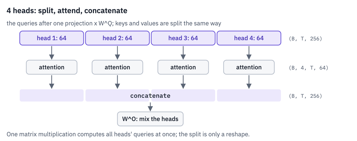
The cutting is a reshape, and it is the least intuitive line of the whole model, so watch it on numbers you can follow: two tokens with eight entries each, numbered 0 to 15, split into two heads of four.
tiny = torch.arange(16.0).reshape(1, 2, 8)  # (B=1, T=2, d_model=8)
print(tiny)

split = tiny.view(1, 2, 2, 4)  # (B, T, h, d_k): each vector cut into 2 pieces of 4
heads_first = split.transpose(1, 2)  # (B, h, T, d_k): heads become a batch dimension
print(heads_first)
tensor([[[ 0.,  1.,  2.,  3.,  4.,  5.,  6.,  7.],
         [ 8.,  9., 10., 11., 12., 13., 14., 15.]]])
tensor([[[[ 0.,  1.,  2.,  3.],
          [ 8.,  9., 10., 11.]],

         [[ 4.,  5.,  6.,  7.],
          [12., 13., 14., 15.]]]])
Head 0 got the first four entries of every token (0–3 and 8–11), head 1 the last four. After transpose the heads stand in the batch dimension, so attention runs on all of them at once without knowing that heads exist. Gluing them back is the same in reverse, transpose then reshape. The class:
class MultiHeadAttention(nn.Module):
    def __init__(self, d_model, n_heads):
        super().__init__()
        self.n_heads = n_heads
        self.d_k = d_model // n_heads
        self.w_q = nn.Linear(d_model, d_model)  # the queries of all heads at once
        self.w_k = nn.Linear(d_model, d_model)
        self.w_v = nn.Linear(d_model, d_model)
        self.w_o = nn.Linear(d_model, d_model)  # mixes the heads back together
        self.weights = None  # the last attention weights, kept for plotting

    def split_heads(self, x):
        batch, length, _ = x.shape
        x = x.view(batch, length, self.n_heads, self.d_k)  # (B, T, h, d_k)
        return x.transpose(1, 2)  # (B, h, T, d_k)

    def forward(self, x_query, x_key_value, mask=None):
        q = self.split_heads(self.w_q(x_query))
        k = self.split_heads(self.w_k(x_key_value))
        v = self.split_heads(self.w_v(x_key_value))
        out, self.weights = attention(q, k, v, mask)  # (B, h, T, d_k)
        batch, _, length, _ = out.shape
        out = out.transpose(1, 2).reshape(batch, length, -1)  # concatenate: (B, T, d_model)
        return self.w_o(out)
The queries come from x_query and the keys and values from x_key_value. For self-attention, the caller passes the same sequence twice; for cross-attention, the Russian side and the encoder’s memory.
PyTorch has a ready-made nn.MultiheadAttention. It stores the three input projections as one matrix, so copy our weights into it and compare the outputs:
ours = MultiHeadAttention(D_MODEL, N_HEADS)
theirs = nn.MultiheadAttention(D_MODEL, N_HEADS, batch_first=True)

with torch.no_grad():
    in_weights = [ours.w_q.weight, ours.w_k.weight, ours.w_v.weight]
    in_biases = [ours.w_q.bias, ours.w_k.bias, ours.w_v.bias]
    theirs.in_proj_weight.copy_(torch.cat(in_weights))
    theirs.in_proj_bias.copy_(torch.cat(in_biases))
    theirs.out_proj.weight.copy_(ours.w_o.weight)
    theirs.out_proj.bias.copy_(ours.w_o.bias)

x = torch.randn(2, 9, D_MODEL)
mask = causal_mask(9)
out_ours = ours(x, x, mask)
out_theirs, _ = theirs(x, x, x, attn_mask=mask[0, 0])
assert torch.allclose(out_ours, out_theirs, atol=1e-5)

n_params = sum(p.numel() for p in ours.parameters())
print("same output as nn.MultiheadAttention;", n_params, "parameters = 4 × (d² + d)")
same output as nn.MultiheadAttention; 263168 parameters = 4 × (d² + d)8. Word order
Attention has a blind spot: it doesn’t know where anything is. Each output is a weighted average over the other positions, and an average doesn’t depend on the order of its terms. Shuffle the words of the sentence, and the outputs are shuffled the same way, with nothing else changed:
x = embedding(src_ids) * math.sqrt(D_MODEL)  # (1, T, d_model)
shuffle = torch.randperm(x.shape[1])

out = ours(x, x)
out_shuffled = ours(x[:, shuffle], x[:, shuffle])
assert torch.allclose(out[:, shuffle], out_shuffled, atol=1e-5)

shuffled_tokens = [encoding.tokens[i] for i in shuffle.tolist()]
token_chips([encoding.tokens, shuffled_tokens], labels=["sentence", "shuffled"])
plt.show()

To attention alone, these two rows are the same sentence. For a translator that’s fatal: she said the researcher was exhausted and the researcher said she was exhausted are different sentences with different translations. So the position has to be written into the vector itself. The paper adds a positional encoding: for position \(pos\) and the pair of entries \(2i\) and \(2i+1\),
\[PE_{(pos,\,2i)} = \sin\!\left(\frac{pos}{10000^{2i/d_{\text{model}}}}\right), \qquad PE_{(pos,\,2i+1)} = \cos\!\left(\frac{pos}{10000^{2i/d_{\text{model}}}}\right).\]- \(pos\) is the position, \(0, 1, 2, \dots\)
- Each pair of entries is a sine and a cosine of the same frequency \(\omega_i = 10000^{-2i/d_{\text{model}}}\). The frequencies fall geometrically from 1 to \(1/10000\): the first pairs turn quickly from one position to the next, like the second hand of a clock; the last ones barely move over a whole sentence, like the hour hand. Together they give every position a distinct pattern, the way the hands of a clock tell every minute of a day apart.
- The values lie between \(-1\) and \(1\), the size of the scaled embeddings they are added to (section 3).
def positional_encoding(max_len, d_model):
    positions = torch.arange(max_len).unsqueeze(1)  # (max_len, 1)
    frequencies = 10_000 ** (-torch.arange(0, d_model, 2) / d_model)  # (d_model / 2,)
    angles = positions * frequencies  # (max_len, d_model / 2)
    pe = torch.zeros(max_len, d_model)
    pe[:, 0::2] = torch.sin(angles)  # even entries
    pe[:, 1::2] = torch.cos(angles)  # odd entries
    return pe


pe = positional_encoding(256, D_MODEL)
Why sines and cosines, rather than, say, the position number itself? Because of the identity \(\sin a \sin b + \cos a \cos b = \cos(a - b)\). Apply it to every pair of entries, and the dot product of the encodings of positions \(p\) and \(p + k\) is
\[PE_p \cdot PE_{p+k} = \sum_i \cos(k\,\omega_i),\]which depends only on the distance \(k\), not on where in the sentence the pair is. Attention compares positions through dot products, so “the word two positions back” looks the same to it at the start of a sentence and at the end. Check it from three starting positions:
offsets = range(64)
curves = {}
for start in [0, 20, 100]:
    curves[start] = [(pe[start] @ pe[start + offset]).item() for offset in offsets]

assert np.allclose(curves[0], curves[20], atol=1e-3)
assert np.allclose(curves[0], curves[100], atol=1e-3)

fig, axes = plt.subplots(1, 2, figsize=(10, 3.6), gridspec_kw={"width_ratios": [1.4, 1]})
axes[0].imshow(pe[:64].T, cmap="PuOr", aspect="auto", vmin=-1, vmax=1)
axes[0].set_xlabel("position")
axes[0].set_ylabel("entry of the vector")
axes[0].set_title("Positional encoding: fast hands at the top")
axes[0].grid(False)
styles = {0: "-", 20: "--", 100: ":"}  # the curves overlap; line styles tell them apart
for start, dots in curves.items():
    axes[1].plot(offsets, dots, linestyle=styles[start], label=f"from position {start}")
axes[1].set_xlabel("distance k")
axes[1].set_ylabel("PE(p) · PE(p + k)")
axes[1].set_title("Similarity depends only on distance")
axes[1].legend()
plt.tight_layout()
plt.show()
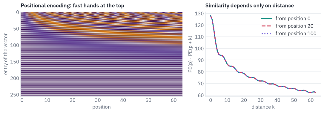
On the left, every column is one position’s vector: the top rows alternate fast, the bottom rows hardly change. On the right, the three curves lie on top of each other, and the similarity falls as positions move apart. Llama and DeepSeek use a descendant of this idea, rotary position embeddings (RoPE), which apply the rotation inside attention itself; lesson 5 builds them.
9. The rest of a layer
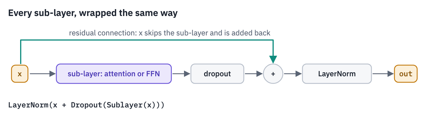
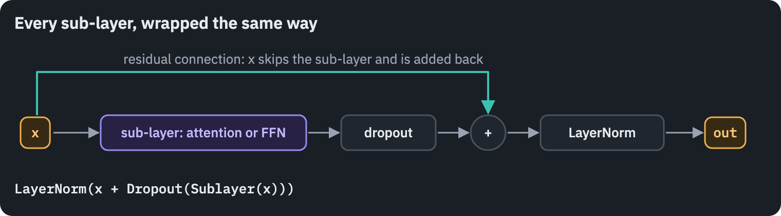
Attention is one of two sub-layers in a Transformer layer; the other is a feed-forward network. Both sit inside the same wrapper:
Feed-forward network. Attention moves information between positions; the feed-forward network then works on what each position has gathered, every position separately and with the same weights:
\[\operatorname{FFN}(\mathbf{x}) = \max(0,\ \mathbf{x} W_1 + \mathbf{b}_1)\, W_2 + \mathbf{b}_2,\]with \(W_1\) of shape \((d_{\text{model}}, d_{\text{ff}})\) and \(W_2\) of shape \((d_{\text{ff}}, d_{\text{model}})\): the vector is widened four times, passed through ReLU, \(\max(0, \cdot)\), which zeroes the negative entries, and narrowed back. The ReLU is what makes it more than a matrix multiplication: without it, \(W_1 W_2\) would collapse into a single matrix. Studies of trained models suggest these layers act as a kind of memory: their first matrix recognizes patterns in the vector and the second adds what is associated with them (Geva et al., 2021).
class FeedForward(nn.Module):
    def __init__(self, d_model, d_ff):
        super().__init__()
        self.linear1 = nn.Linear(d_model, d_ff)  # widen
        self.linear2 = nn.Linear(d_ff, d_model)  # and narrow back

    def forward(self, x):
        return self.linear2(torch.relu(self.linear1(x)))


feed_forward = FeedForward(D_MODEL, D_FF)
print("feed-forward:", sum(p.numel() for p in feed_forward.parameters()), "parameters")
print("attention:   ", sum(p.numel() for p in ours.parameters()), "parameters")
feed-forward: 525568 parameters
attention:    263168 parameters
Two thirds of an encoder layer’s parameters sit in the feed-forward network, not in attention.
Residual connection. Every sub-layer’s output is added to its input, \(\mathbf{x} + \operatorname{Sublayer}(\mathbf{x})\) (He et al., 2016). A sub-layer then only has to learn a correction to what is already there, rather than rebuild the whole vector. And during training, the gradient flows back through the “+” undiminished, however many layers are stacked. One useful way to picture the result is a residual stream (Elhage et al., 2021): a vector per token that runs from the embedding to the output, with every sub-layer reading from it and adding its contribution back. Among other things, the stream carries the input embedding all the way to the top, which matters more than you’d think in section 11.
Layer normalization (Ba et al., 2016) keeps the stream’s numbers in a stable range, however much the sub-layers add. It rescales every vector to mean 0 and variance 1, then lets the model choose its own scale and shift:
\[\operatorname{LayerNorm}(\mathbf{x}) = \boldsymbol{\gamma} \odot \frac{\mathbf{x} - \mu}{\sqrt{\sigma^2 + \epsilon}} + \boldsymbol{\beta}, \qquad \mu = \frac{1}{d}\sum_i x_i, \quad \sigma^2 = \frac{1}{d}\sum_i (x_i - \mu)^2.\]\(\mu\) and \(\sigma^2\) are the mean and variance of the vector’s own entries; \(\boldsymbol{\gamma}\) and \(\boldsymbol{\beta}\) are learned vectors of length \(d_{\text{model}}\), starting at 1 and 0; \(\epsilon\) prevents division by zero; \(\odot\) multiplies entry by entry. Written out and compared with PyTorch’s:
def layer_norm(x, gamma, beta, eps=1e-5):
    mean = x.mean(dim=-1, keepdim=True)
    variance = x.var(dim=-1, keepdim=True, unbiased=False)
    return gamma * (x - mean) / torch.sqrt(variance + eps) + beta


norm = nn.LayerNorm(D_MODEL)
x = torch.randn(2, 9, D_MODEL) * 3 + 1  # vectors with mean 1 and standard deviation 3
normalized = layer_norm(x, norm.weight, norm.bias)
assert torch.allclose(normalized, norm(x), atol=1e-5)

before, after = x[0, 0], normalized[0, 0]  # one vector
print("before: mean", round(before.mean().item(), 2), "std", round(before.std().item(), 2))
print("after:  mean", round(after.mean().item(), 2), "std", round(after.std().item(), 2))
print("same as nn.LayerNorm; from here on we use PyTorch's")
before: mean 1.22 std 2.85
after:  mean 0.0 std 1.0
same as nn.LayerNorm; from here on we use PyTorch's
The 2017 paper puts the normalization after the addition, \(\operatorname{LayerNorm}(\mathbf{x} + \operatorname{Sublayer}(\mathbf{x}))\): the “add & norm” boxes of the diagram. Most models since put it before the sub-layer instead; lesson 5 measures the difference. Last, dropout with probability \(0.1\) on every sub-layer’s output and on the embeddings: during training, random entries are set to zero (and the rest scaled up to compensate), so the model can’t come to rely on any single one.
10. The whole model
An encoder layer is self-attention and a feed-forward network, each in the wrapper from the picture above. Read forward as two lines of the formula \(\operatorname{LayerNorm}(\mathbf{x} + \operatorname{Dropout}( \operatorname{Sublayer}(\mathbf{x})))\):
class EncoderLayer(nn.Module):
    def __init__(self, d_model, n_heads, d_ff, dropout):
        super().__init__()
        self.self_attention = MultiHeadAttention(d_model, n_heads)
        self.feed_forward = FeedForward(d_model, d_ff)
        self.norm1 = nn.LayerNorm(d_model)
        self.norm2 = nn.LayerNorm(d_model)
        self.dropout = nn.Dropout(dropout)

    def forward(self, x, src_mask):
        x = self.norm1(x + self.dropout(self.self_attention(x, x, src_mask)))
        x = self.norm2(x + self.dropout(self.feed_forward(x)))
        return x
A decoder layer has one more sub-layer between the two: cross-attention, whose queries come from the Russian side and whose keys and values come from the encoder’s memory. Its self-attention gets the causal mask; its cross-attention gets the source’s padding mask, so that no Russian token attends to English padding.
class DecoderLayer(nn.Module):
    def __init__(self, d_model, n_heads, d_ff, dropout):
        super().__init__()
        self.self_attention = MultiHeadAttention(d_model, n_heads)
        self.cross_attention = MultiHeadAttention(d_model, n_heads)
        self.feed_forward = FeedForward(d_model, d_ff)
        self.norm1 = nn.LayerNorm(d_model)
        self.norm2 = nn.LayerNorm(d_model)
        self.norm3 = nn.LayerNorm(d_model)
        self.dropout = nn.Dropout(dropout)

    def forward(self, x, memory, src_mask, tgt_mask):
        x = self.norm1(x + self.dropout(self.self_attention(x, x, tgt_mask)))
        x = self.norm2(x + self.dropout(self.cross_attention(x, memory, src_mask)))
        x = self.norm3(x + self.dropout(self.feed_forward(x)))
        return x
The decoder is trained with teacher forcing: it reads the correct Russian sentence, shifted one position to the right behind a <bos> (“beginning of sentence”) token, and at every position predicts the next token. Thanks to the causal mask, one pass over the sentence trains all positions at once, and none of them can peek at its answer.
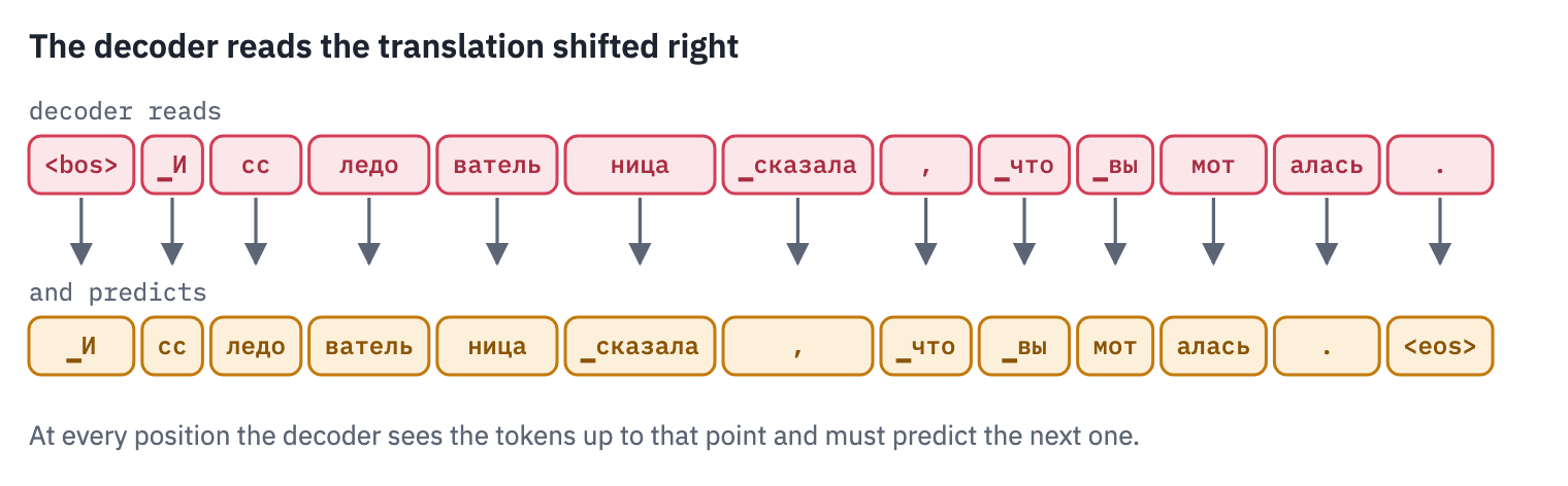
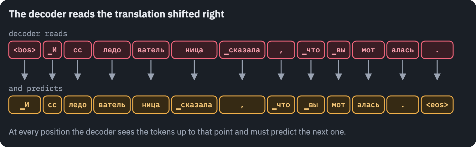 followed by the Russian tokens and is trained to predict, at every position, the next token, ending with
The full model puts it together. One matrix \(E\) serves three times: as the source embedding, as the target embedding (lesson 1 built one shared vocabulary for both languages) and as the output layer. Besides saving parameters, tying the output layer to the embedding tends to improve language models (Press and Wolf, 2017). The class has three methods besides forward: embed turns ids into vectors with positions, encode runs the encoder, and decode runs the decoder and returns the scores. Keeping them separate lets us call the encoder once and the decoder many times when translating.
class Transformer(nn.Module):
    def __init__(
        self, vocab_size, d_model, n_heads, d_ff, n_layers, dropout, pad_id, max_len=256
    ):
        super().__init__()
        self.d_model = d_model
        self.pad_id = pad_id
        self.embedding = nn.Embedding(vocab_size, d_model)
        nn.init.normal_(self.embedding.weight, mean=0.0, std=d_model**-0.5)
        # the positional encoding is fixed, not trained: a buffer, not a parameter
        self.register_buffer("pe", positional_encoding(max_len, d_model))
        self.encoder = nn.ModuleList(
            [EncoderLayer(d_model, n_heads, d_ff, dropout) for _ in range(n_layers)]
        )
        self.decoder = nn.ModuleList(
            [DecoderLayer(d_model, n_heads, d_ff, dropout) for _ in range(n_layers)]
        )
        self.dropout = nn.Dropout(dropout)

    def embed(self, ids):
        x = self.embedding(ids) * math.sqrt(self.d_model) + self.pe[: ids.shape[1]]
        return self.dropout(x)

    def encode(self, src):
        src_mask = padding_mask(src, self.pad_id)
        x = self.embed(src)
        for layer in self.encoder:
            x = layer(x, src_mask)
        return x  # the memory: (B, T_src, d_model)

    def decode(self, tgt, memory, src):
        src_mask = padding_mask(src, self.pad_id)
        tgt_mask = padding_mask(tgt, self.pad_id) + causal_mask(tgt.shape[1], tgt.device)
        x = self.embed(tgt)
        for layer in self.decoder:
            x = layer(x, memory, src_mask, tgt_mask)
        return x @ self.embedding.weight.T  # scores for every token: (B, T_tgt, |V|)

    def forward(self, src, tgt):
        return self.decode(tgt, self.encode(src), src)


model = Transformer(VOCAB_SIZE, D_MODEL, N_HEADS, D_FF, N_LAYERS, DROPOUT, PAD).to(device)
print(sum(p.numel() for p in model.parameters()), "parameters")
9625600 parametersBefore using the model, walk a sentence through it by hand, method by method, and watch the shapes. This is the architecture diagram from section 2, run on our sentence:
src = torch.tensor([tokenizer.encode(EN_EXAMPLE).ids], device=device)
tgt = torch.tensor([[BOS] + tokenizer.encode(RU_EXAMPLE).ids], device=device)

steps = []
model.eval()
with torch.no_grad():
    x = model.embed(src)
    steps.append(("English ids → vectors + positions", tuple(x.shape)))
    for i, layer in enumerate(model.encoder):
        x = layer(x, padding_mask(src, PAD))
        steps.append((f"encoder layer {i + 1}", tuple(x.shape)))
    memory = x

    y = model.embed(tgt)
    steps.append(("Russian ids → vectors + positions", tuple(y.shape)))
    tgt_mask = padding_mask(tgt, PAD) + causal_mask(tgt.shape[1], device)
    for i, layer in enumerate(model.decoder):
        y = layer(y, memory, padding_mask(src, PAD), tgt_mask)
        steps.append((f"decoder layer {i + 1}, reading the memory", tuple(y.shape)))
    scores = y @ model.embedding.weight.T
    steps.append(("× Eᵀ: a score for every token", tuple(scores.shape)))

table(pd.DataFrame(steps, columns=["step", "shape (B, T, ·)"]))
| step | shape (B, T, ·) |
|---|---|
| English ids → vectors + positions | (1, 9, 256) |
| encoder layer 1 | (1, 9, 256) |
| encoder layer 2 | (1, 9, 256) |
| encoder layer 3 | (1, 9, 256) |
| Russian ids → vectors + positions | (1, 13, 256) |
| decoder layer 1, reading the memory | (1, 13, 256) |
| decoder layer 2, reading the memory | (1, 13, 256) |
| decoder layer 3, reading the memory | (1, 13, 256) |
| × Eᵀ: a score for every token | (1, 13, 16000) |
Every layer keeps the shape it receives: one vector of 256 numbers per token. The encoder never sees the Russian side, and the decoder sees the English side only through the memory. Only the last step leaves the width of the model, and there every Russian position gets one score for each of the sixteen thousand tokens.
Where do the parameters live? Group them by the part of the model they belong to:
parts = collections.Counter()
for name, parameter in model.named_parameters():
    if name.startswith("embedding"):
        part = "embedding E, shared"
    elif "norm" in name:
        part = "layer norms"
    else:
        stack = name.split(".")[0]  # "encoder" or "decoder"
        sub_layer = name.split(".")[2]  # self_attention, cross_attention or feed_forward
        part = stack + ": " + sub_layer.replace("_", "-")
    parts[part] += parameter.numel()

colors = []  # the course's concept colors: amber embedding, teal encoder, rose decoder
for part in parts:
    if part.startswith("embedding"):
        colors.append(COLORS["data"])
    elif part.startswith("encoder"):
        colors.append(COLORS["enc"])
    elif part.startswith("decoder"):
        colors.append(COLORS["dec"])
    else:
        colors.append(COLORS["muted"])

bars(dict(parts), colors=colors, title="Where the parameters live")
plt.show()
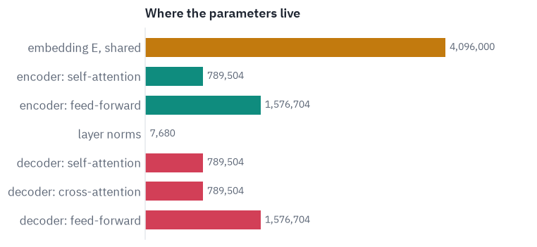
The shared embedding is the largest single part, which is why lesson 1 weighed every extra token against its row. Every count follows from the shapes, so the total is a formula, with \(d = d_{\text{model}}\):
\[\underbrace{\lvert\mathcal{V}\rvert\, d}_{\text{embedding}} + N\big(\underbrace{4(d^2 + d)}_{\text{attention}} + \underbrace{2 d d_{\text{ff}} + d_{\text{ff}} + d}_{\text{ feed-forward}} + \underbrace{2 \cdot 2d}_{\text{norms}}\big) + N\big(2 \cdot 4(d^2 + d) + 2 d d_{\text{ff}} + d_{\text{ff}} + d + 3 \cdot 2d\big):\]the embedding, \(N\) encoder layers, and \(N\) decoder layers with their two attentions and three norms. An attention has four \(d \times d\) matrices with biases; a feed-forward network two matrices of \(d \times d_{\text{ff}}\) with biases; a norm has \(\boldsymbol{\gamma}\) and \(\boldsymbol{\beta}\).
def count_parameters(vocab_size, d, d_ff, n_layers):
    attention_params = 4 * (d * d + d)
    feed_forward_params = 2 * d * d_ff + d_ff + d
    encoder_layer = attention_params + feed_forward_params + 2 * 2 * d
    decoder_layer = 2 * attention_params + feed_forward_params + 3 * 2 * d
    return vocab_size * d + n_layers * encoder_layer + n_layers * decoder_layer


by_formula = count_parameters(VOCAB_SIZE, D_MODEL, D_FF, N_LAYERS)
assert by_formula == sum(p.numel() for p in model.parameters())
print("the formula matches the model:", by_formula)
the formula matches the model: 962560011. A first run, and a parrot
Make a batch of real sentence pairs and run the model. The source is the English ids; the decoder reads <bos> and the Russian ids, and the target is the Russian ids followed by <eos>, “end of sentence”.
def make_batch(pairs):
    src = pad_batch([tokenizer.encode(en).ids for en, _ in pairs])
    tgt_in = pad_batch([[BOS] + tokenizer.encode(ru).ids for _, ru in pairs])
    tgt_out = pad_batch([tokenizer.encode(ru).ids + [EOS] for _, ru in pairs])
    return src.to(device), tgt_in.to(device), tgt_out.to(device)


pairs = list(zip(valid.en[:64], valid.ru[:64]))
src, tgt_in, tgt_out = make_batch(pairs)

model.eval()  # no dropout while we measure
with torch.no_grad():
    logits = model(src, tgt_in)
print("source:", tuple(src.shape))
print("decoder input:", tuple(tgt_in.shape))
print("scores:", tuple(logits.shape))
source: (64, 38)
decoder input: (64, 42)
scores: (64, 42, 16000)
The model will be trained to make the correct next token likely. Its loss is the course’s cross-entropy, the average of \(-\log\) of the probability it gives the right token:
\[\mathcal{L}(\theta) = -\frac{1}{m} \sum_{t=1}^{m} \log p_\theta(y_t \mid y_{<t}, \mathbf{x}),\]where the probabilities come from the scores by softmax. In terms of the scores \(z_j\) at one position, the loss there is \(\log \sum_j e^{z_j} - z_{\text{target}}\).
Before training, we can predict its value. Section 3 set the scores up to be roughly independent, with mean 0 and a variance \(\sigma^2\) of about 1. The target’s score is then 0 on average, and a sum over sixteen thousand tokens is close to its expected value, \(\lvert\mathcal{V}\rvert\,\mathbb{E}[e^{z}] = \lvert\mathcal{V}\rvert\, e^{\sigma^2/2}\) (the mean of \(e^z\) when \(z\) is normal). So
\[\mathcal{L}_{\text{init}} \approx \log\lvert\mathcal{V}\rvert + \frac{\sigma^2}{2}.\]The \(\log\lvert\mathcal{V}\rvert\) part is the loss of a model that gives every token the same probability, the most honest thing a model can do before it has learned anything. Measure it:
real = tgt_out != PAD  # positions that hold real target tokens
loss = F.cross_entropy(logits[real], tgt_out[real]).item()
sigma2 = logits[real].var().item()

print("measured loss:     ", round(loss, 3))
print("log|V| + sigma²/2: ", round(math.log(VOCAB_SIZE) + sigma2 / 2, 3))
measured loss:      11.603
log|V| + sigma²/2:  10.186
More than a whole unit too high. A gap like this usually means a bug, so look at what the model predicts: its top token at every position, under the token it has just read.
predicted = logits.argmax(dim=-1)
same_as_input = (predicted[real] == tgt_in[real]).float().mean().item()
print(f"top prediction = the token the decoder just read: {same_as_input:.1%} of positions")

n = int(real[0].sum())  # the first sentence of the batch
read = [tokenizer.id_to_token(i) for i in tgt_in[0, :n].tolist()]
guessed = [tokenizer.id_to_token(i) for i in predicted[0, :n].tolist()]
token_chips([read, guessed], labels=["reads", "predicts"])
plt.show()
top prediction = the token the decoder just read: 100.0% of positions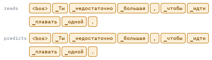
The untrained model is a parrot: at every position it predicts the token it has just read. That’s not a bug, and the explanation joins two sections of this lesson. The residual stream carries the input embedding \(\sqrt{d_{\text{model}}}\,\mathbf{e}_t\) up through every layer, so the final vector still points partly along \(\mathbf{e}_t\). And the output layer is the same matrix \(E\), so the score of token \(t\) is the dot product of that vector with \(\mathbf{e}_t\) itself. Here are all sixteen thousand scores at one position:
position = 3  # the fourth position of the first sentence
scores_here = logits[0, position].cpu()
just_read = tgt_in[0, position].item()

fig, ax = plt.subplots(figsize=(6.4, 2.8))
ax.hist(scores_here, bins=80, color=COLORS["muted"])
ax.set_yscale("log")
ax.axvline(scores_here[just_read], color=COLORS["data"], linewidth=2)
label_height = ax.get_ylim()[1] / 4
ax.text(scores_here[just_read], label_height, " " + tokenizer.id_to_token(just_read))
ax.set_xlabel("score")
ax.set_ylabel("tokens")
ax.set_title("One score far from all the others: the token just read")
plt.show()
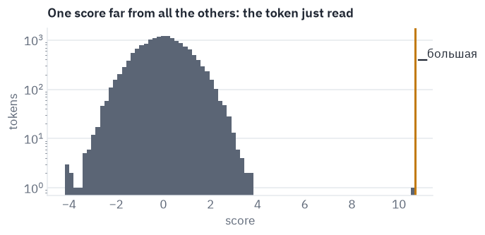
The bulk of the scores sits around 0, as section 3 planned, and one token, the one just read, stands far to the right. Measured over the whole batch:
is_just_read = F.one_hot(tgt_in, VOCAB_SIZE).bool()  # (B, T, |V|): True at the token read
own_scores = logits[is_just_read & real.unsqueeze(-1)]
print("score of the token just read, on average:", round(own_scores.mean().item(), 2))
print("spread of all scores, std:", round(logits[real].std().item(), 2))
score of the token just read, on average: 10.98
spread of all scores, std: 1.01
One score in sixteen thousand, far above all the others, is exactly what pushes \(\log\sum_j e^{z_j}\) up. Take it out at every position, as if that token weren’t in the vocabulary, and check the two parts of the loss separately: the log of the sum, which the formula now predicts as \(\log(\lvert\mathcal{V}\rvert - 1) + \sigma^2/2\), and the score of the right token, which it assumes to be 0 on average.
# drop the score of the token just read; skip the rare positions whose answer is that token
without_own = logits.masked_fill(is_just_read, float("-inf"))
keep = real & (tgt_in != tgt_out)

others = without_own[keep]  # (positions, |V|)
log_sum = torch.logsumexp(others, dim=-1).mean().item()
rows_index = torch.arange(len(others))
right_score = others[rows_index, tgt_out[keep]].mean().item()  # each row's right token
sigma2_others = others[torch.isfinite(others)].var().item()
expected = math.log(VOCAB_SIZE - 1) + sigma2_others / 2

print("log of the sum, measured:   ", round(log_sum, 4))
print("log(|V| - 1) + sigma²/2:    ", round(expected, 4))
print("score of the right token:   ", round(right_score, 3))
assert abs(log_sum - expected) < 0.02
log of the sum, measured:    10.1796
log(|V| - 1) + sigma²/2:     10.1818
score of the right token:    -0.204
Now the formula holds to the second decimal. The score of the right token is near 0 but not exactly: a different random initialization moves it a little above or below, and the loss with it. The parrot is the big effect, and the first steps of training break the habit, because it is wrong almost everywhere: a translation rarely repeats a token twice in a row.
12. Can it learn?
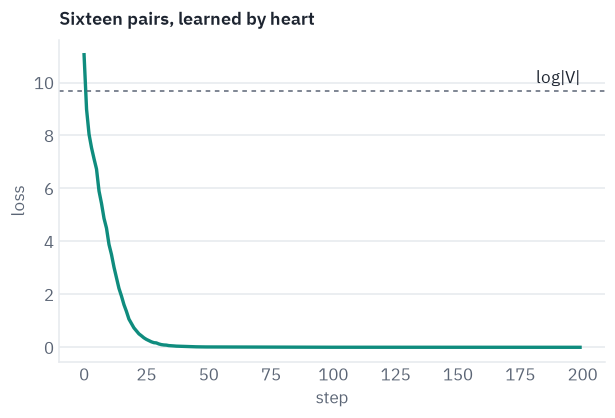
Before spending an hour of GPU time on training (lesson 3), make sure the model can learn at all. The cheapest test is to teach it a handful of sentence pairs by heart: a model that can’t memorize sixteen pairs has a bug somewhere. Karpathy (2019) calls this step “overfit one batch”.
One detail: lesson 1 kept groups of linked pairs together, so the validation set holds several translations of some English sentences. Nobody can memorize two answers to one question, so we take one pair per English sentence, plus our own sentence. The training loop is the simplest possible; lesson 3 explains each of its parts and adds the ones a real run needs.
distinct = valid.drop_duplicates("en")
lesson_pairs = [(EN_EXAMPLE, RU_EXAMPLE)] + list(zip(distinct.en[:15], distinct.ru[:15]))
src, tgt_in, tgt_out = make_batch(lesson_pairs)

model.train()  # dropout on, as in real training
optimizer = torch.optim.Adam(model.parameters(), lr=1e-3)

losses = []
start = time.perf_counter()
for _ in range(200):
    logits = model(src, tgt_in)
    flat_logits = logits.reshape(-1, VOCAB_SIZE)  # every position of every sentence
    loss = F.cross_entropy(flat_logits, tgt_out.reshape(-1), ignore_index=PAD)
    optimizer.zero_grad()  # forget the previous step's gradients
    loss.backward()  # compute new ones, through every layer
    optimizer.step()  # move every parameter a little against its gradient
    losses.append(loss.item())

seconds = round(time.perf_counter() - start, 1)
print(len(losses), "steps in", seconds, "s")
print("loss:", round(losses[0], 2), "->", round(losses[-1], 4))
200 steps in 12.9 s
loss: 11.05 -> 0.0017fig, ax = plt.subplots()
ax.plot(losses, color=COLORS["enc"])
ax.axhline(math.log(VOCAB_SIZE), color=COLORS["muted"], linestyle=(0, (3, 3)), linewidth=1)
ax.text(len(losses) - 1, math.log(VOCAB_SIZE) + 0.3, "log|V|", ha="right")
ax.set_xlabel("step")
ax.set_ylabel("loss")
ax.set_title("Sixteen pairs, learned by heart")
plt.show()
To translate, the model writes one token at a time: encode the English sentence once, then repeatedly feed the decoder everything written so far and append its top prediction, until it predicts <eos>. This is greedy decoding; lesson 3 shows why it isn’t the best way to decode, and does better.
def translate_greedy(model, sentence, max_tokens=60):
    model.eval()
    src = torch.tensor([tokenizer.encode(sentence).ids], device=device)
    written = [BOS]
    with torch.no_grad():
        memory = model.encode(src)  # the English side, once
        for _ in range(max_tokens):
            tgt = torch.tensor([written], device=device)
            scores = model.decode(tgt, memory, src)[0, -1]  # scores for the next token
            next_id = scores.argmax().item()
            if next_id == EOS:
                break
            written.append(next_id)
    return tokenizer.decode(written[1:])


rows = []
for en, ru in lesson_pairs:
    output = translate_greedy(model, en)
    rows.append({"English": en, "model's Russian": output, "exact": output == ru})
memorized = pd.DataFrame(rows)
print(memorized.exact.sum(), "of", len(memorized), "translations reproduced exactly")
assert memorized.exact.all()
table(memorized.head(6))
16 of 16 translations reproduced exactly| English | model's Russian | exact |
|---|---|---|
| The researcher said she was exhausted. | Исследовательница сказала, что вымоталась. | True |
| You are not old enough to go swimming by yourself. | Ты недостаточно большая, чтобы идти плавать одной. | True |
| You are made to be a poet. | Ты прирождённый поэт. | True |
| You are the next in line for promotion. | Вы — следующий в очереди на повышение. | True |
| You are the master of your own destiny. | Ты хозяин своей собственной судьбы. | True |
| You are wearing your socks inside out. | У тебя носки наизнанку. | True |
Every pair comes back exactly, our sentence with its three feminine forms included. The model memorized, though; it hasn’t learned to translate anything it hasn’t seen. Its attention shows it. Here is the cross-attention of the last decoder layer while it writes our sentence, averaged over the four heads: every row is a Russian token, and its cells show how much it took from each English token.
src = torch.tensor([tokenizer.encode(EN_EXAMPLE).ids], device=device)
tgt = torch.tensor([[BOS] + tokenizer.encode(RU_EXAMPLE).ids], device=device)
with torch.no_grad():
    model(src, tgt)  # the attention modules keep their last weights

cross = model.decoder[-1].cross_attention.weights[0].mean(dim=0).cpu()  # (T_ru, T_en)
en_tokens = tokenizer.encode(EN_EXAMPLE).tokens
ru_read = ["<bos>"] + tokenizer.encode(RU_EXAMPLE).tokens

heatmap(
    cross,
    rows=ru_read,
    cols=en_tokens,
    vmax=1,
    title="Cross-attention after memorizing: nearly flat",
    xlabel="English (keys)",
    ylabel="Russian (queries)",
)
plt.show()

print("uniform weight over the English tokens:", round(1 / len(en_tokens), 3))
print("largest weight in the map:", round(cross.max().item(), 3))
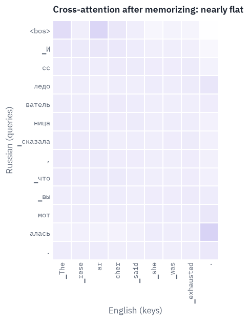
uniform weight over the English tokens: 0.111
largest weight in the map: 0.259
Nearly flat: almost every Russian token spreads its attention evenly across the English sentence. Memorizing sixteen pairs doesn’t require knowing which English word a Russian word translates; the model can get by on what each sentence looks like as a whole. Lesson 3 trains on half a million pairs, where that shortcut no longer works, and we will come back to this picture to see whether сказала has learned to look at she.
13. Our code, at the size of a real model
Back to the table of section 1. opus-mt-en-ru has the shape of the 2017 base model, and our class implements that architecture. Build it with opus-mt-en-ru’s numbers instead of ours, and count:
opus = configs["opus-mt-en-ru (2020)"]
opus_sized = Transformer(
    vocab_size=opus["vocab_size"],
    d_model=opus["d_model"],
    n_heads=opus["encoder_attention_heads"],
    d_ff=opus["encoder_ffn_dim"],
    n_layers=opus["encoder_layers"],
    dropout=0.1,
    pad_id=opus["pad_token_id"],
)
opus_sized_params = sum(p.numel() for p in opus_sized.parameters())
print("our class at opus-mt-en-ru's size:", opus_sized_params, "parameters")
print(round(opus_sized_params / by_formula, 1), "times the size of our model")
our class at opus-mt-en-ru's size: 76147712 parameters
7.9 times the size of our model
The real model’s weights are a file of about 300 MB. Without downloading it, the Hub tells us its size, and at four bytes per number we can account for nearly every byte. Two differences from our model are known in advance: Marian stores its sinusoidal position tables in the file (one for the encoder and one for the decoder) instead of computing them, and it adds a bias to the output scores.
info = HfApi().model_info("Helsinki-NLP/opus-mt-en-ru", files_metadata=True)
file_size = [f.size for f in info.siblings if f.rfilename == "pytorch_model.bin"][0]

position_tables = 2 * opus["max_position_embeddings"] * opus["d_model"]
output_bias = opus["vocab_size"]
accounted = 4 * (opus_sized_params + position_tables + output_bias)

print("the real file:             ", file_size, "bytes")
print("our parameters and extras: ", accounted, "bytes")
left_over = file_size - accounted
print(f"left over: {left_over} bytes, {left_over / file_size:.3%} of the file")
the real file:              306991893 bytes
our parameters and extras:  306938072 bytes
left over: 53821 bytes, 0.018% of the file
What is left over is the file format itself: the tensors’ names and headers. The translator we will compete with is, number for number, the model you just wrote, at several times our size.
The model’s code is also in the course package, tfs.model, so that later lessons can import it instead of repeating it. Check that it is the same model, weight for weight:
from tfs.model import Transformer as PackagedTransformer

packaged = PackagedTransformer(VOCAB_SIZE, D_MODEL, N_HEADS, D_FF, N_LAYERS, DROPOUT, PAD)
packaged = packaged.to(device)
packaged.load_state_dict(model.state_dict())

src, tgt_in, _ = make_batch(lesson_pairs[:4])
model.eval()
packaged.eval()
with torch.no_grad():
    assert torch.allclose(packaged(src, tgt_in), model(src, tgt_in), atol=1e-5)
print("tfs.model.Transformer is the model of this lesson")
tfs.model.Transformer is the model of this lessonReferences
- Vaswani, A., Shazeer, N., Parmar, N., Uszkoreit, J., Jones, L., Gomez, A. N., Kaiser, Ł., Polosukhin, I. (2017). Attention Is All You Need. NeurIPS.
- Bahdanau, D., Cho, K., Bengio, Y. (2015). Neural Machine Translation by Jointly Learning to Align and Translate. ICLR. Attention itself was invented for translation, three years before the Transformer.
- He, K., Zhang, X., Ren, S., Sun, J. (2016). Deep Residual Learning for Image Recognition. CVPR.
- Ba, J. L., Kiros, J. R., Hinton, G. E. (2016). Layer Normalization.
- Press, O., Wolf, L. (2017). Using the Output Embedding to Improve Language Models. EACL.
- Geva, M., Schuster, R., Berant, J., Levy, O. (2021). Transformer Feed-Forward Layers Are Key-Value Memories. EMNLP.
- Elhage, N. et al. (2021). A Mathematical Framework for Transformer Circuits. Where the “residual stream” comes from.
- Rush, A. (2018). The Annotated Transformer. The paper, line by line, in PyTorch.
- Junczys-Dowmunt, M. et al. (2018). Marian: Fast Neural Machine Translation in C++. ACL.
- Tiedemann, J., Thottingal, S. (2020). OPUS-MT: Building open translation services for the World. EAMT.
- Karpathy, A. (2019). A Recipe for Training Neural Networks.
- Model configurations: GPT-2, opus-mt-en-ru, Llama 3.1 8B, DeepSeek-V3.