Contents
Transformer architectures: from BERT to diffusion · lesson 1 of 15 · all lessons · run on Kaggle · open in Colab · code on GitHub
In October 2019 Google changed the way its search engine reads queries. Its own example was the query “2019 brazil traveler to usa need a visa”. The old system treated the little word to as noise and “returned results about U.S. citizens traveling to Brazil”, which is the other way around.
The new one understood that the traveller goes from Brazil to the US. Google said the model would help with “one in 10 searches in the U.S. in English” and called it “the biggest leap forward in the past five years” [1].
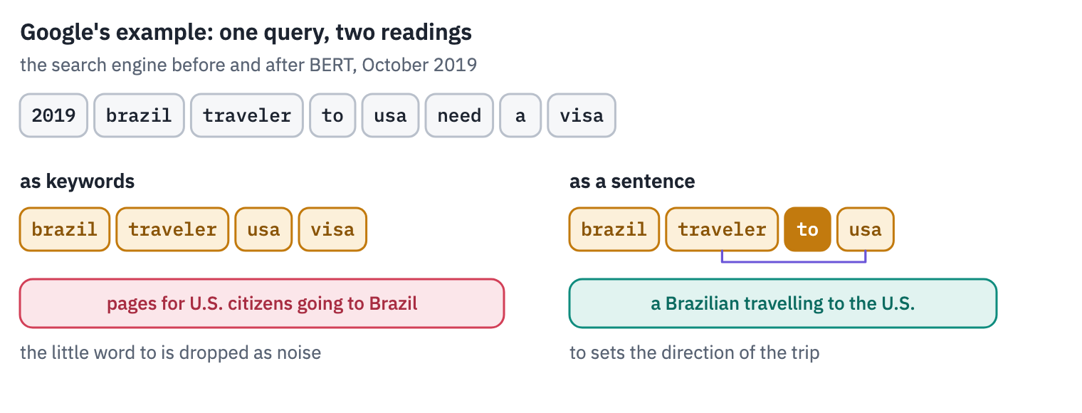
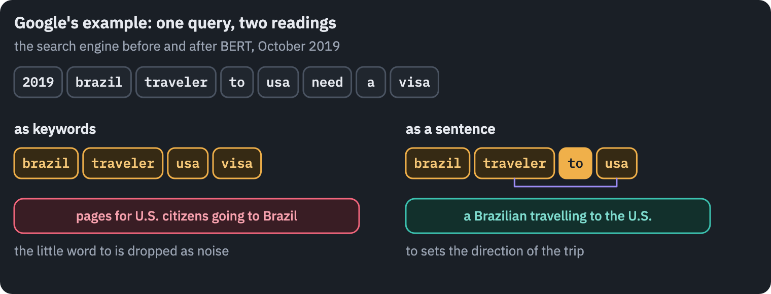
The model was BERT, published by Google a year earlier [2]. It is the Transformer encoder you built in the first course, trained on books and Wikipedia to fill in hidden words, and then taught a task with a few thousand examples.
That recipe, pre-train once and fine-tune for everything, is how most of NLP worked for the next four years, and BERT-sized encoders still sort, tag and search a large part of the world’s text, because they are small, fast and very good at it.
In this lesson you will write BERT yourself, load Google’s weights into your code and check that it gives exactly the same answers as the reference implementation. Then you will ask it what it learned, look at what its attention heads do, and teach it a job that companies pay for: finding personal data in financial documents.
What you’ll do
- See why a language model couldn’t simply read in both directions, and how a mask fixed it.
- Read BERT-base’s blueprint from its config and count where its 110 million parameters live.
- Write BERT in PyTorch, load Google’s weights into it and match Hugging Face’s outputs.
- Mask words the way BERT was trained, and ask it about facts, grammar, negation and gender.
- Look inside its attention: which heads watch the previous word, and why so many watch
[SEP]. - Fine-tune it to find names, addresses and account numbers in long documents, and compare it with regular expressions and with the same network trained without pre-training.
What you need: a GPU. On Kaggle, Settings → Accelerator → GPU; on Colab, Runtime → Change runtime type → T4 GPU.
The notebook downloads BERT-base twice (uncased and cased, 440 MB each) and a dataset of synthetic financial documents, and fine-tunes seven models, most of them on a few hundred documents; on a T4 it runs in about an hour.
Setup
One small helper package, tfs, draws the course’s plots and token chips and knows where the notebook runs (Kaggle, Colab or your own machine). Everything the lesson teaches is written out in the notebook itself.
import importlib.util
import subprocess
import sys

TFS = "git+https://github.com/xmarva/transformers-from-scratch@main"
if importlib.util.find_spec("tfs") is None:
    subprocess.check_call([sys.executable, "-m", "pip", "install", "-q", TFS])

from tfs import env
from tfs.viz import table, token_chips, use_course_style

env.quiet()  # no progress bars or environment warnings in the outputs
SEED = 42
env.seed_everything(SEED)
COLORS = use_course_style()
WORK_DIR = env.work_dir()
import json
import math
import random
import re
import time

import matplotlib.pyplot as plt
import numpy as np
import pandas as pd
import torch
import torch.nn as nn
import torch.nn.functional as F
from datasets import load_dataset
from huggingface_hub import get_safetensors_metadata, hf_hub_download
from IPython.display import HTML, display
from safetensors.torch import load_file
from tfs.viz import heatmap
from transformers import AutoTokenizer, BertForMaskedLM

import warnings

# mixed precision skips a step when a gradient overflows; PyTorch reports it as a warning
warnings.filterwarnings("ignore", message="Detected call of `lr_scheduler.step")
SMOKE = env.smoke()  # CI runs the lesson on a small slice; you run it in full
device = "cuda" if torch.cuda.is_available() else "cpu"
assert device == "cuda" or SMOKE, "This lesson fine-tunes BERT seven times: use a GPU."
if device == "cuda":
    print("GPU:", torch.cuda.get_device_name(0))
GPU: Tesla T41. Reading in both directions
Before BERT, the standard way to give a network some knowledge of language was a table of word vectors, such as word2vec’s: one vector per word, learned from which words appear near which. One vector per word is the problem.
Bank gets the same vector in “the bank raised its rates” and “we sat on the river bank”, and the network that uses it has to work out the difference on its own, from whatever little labelled data it has.
The fix everyone could see was to read the whole sentence first: a vector for bank computed from its neighbours. A language model does exactly that.
It is trained on raw text, which is free and endless, to predict the next word, so its hidden state at every position is a summary of the words before it. In 2018 two models showed how much that summary is worth.
ELMo trained two recurrent language models, one reading left to right and one right to left, and glued their states together[3]. OpenAI’s first GPT trained a Transformer decoder left to right and fine-tuned the whole of it for each task [4].
Both read with one eye closed. In “we sat on the river bank” the word that decides what bank means comes before it, but in “the bank of the river was steep” it comes after, and a left-to-right model sees it too late.
ELMo’s two directions never meet inside the network: each half reads one way, and only their outputs are joined.
Why not train one model that reads both ways at once? Because it would cheat. Devlin and colleagues put it in one sentence: “bidirectional conditioning would allow each word to indirectly ‘see itself’, and the model could trivially predict the target word in a multi-layered context.”
Ask a model to predict word 5 while it can attend to word 5, and it learns to copy. Even if word 5 can’t attend to itself in the first layer, word 6 can, and in the second layer word 5 reads it back from word 6.
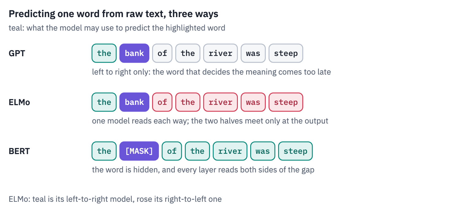
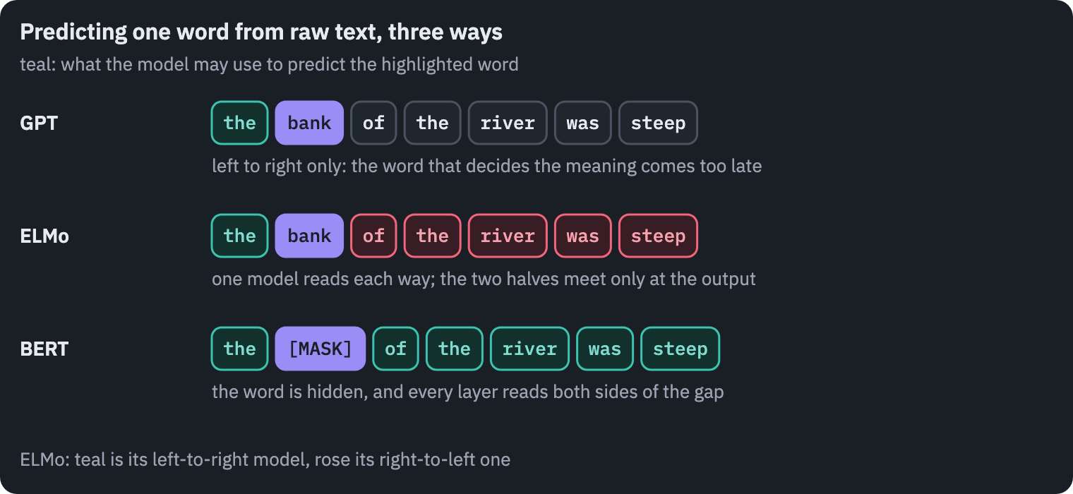
BERT’s answer is old. In 1953 Wilson Taylor proposed measuring how readable a text is by deleting every fifth word and asking people to fill the gaps; he called it the cloze procedure [5].
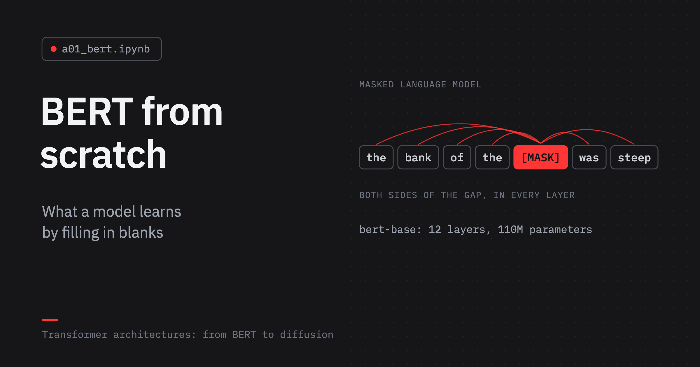
BERT plays the same game. It hides some of the words, replaces them with a special token [MASK] and is trained to restore them.
A hidden word can’t see itself, so every layer can attend to everything else, in both directions. The paper calls this the masked language model (MLM), “inspired by the Cloze task (Taylor, 1953)”.
The price is efficiency. A left-to-right model learns from every word of every sentence; BERT learns only from the 15% it hides.
Google paid for that with compute: BERT-base was trained “on 4 Cloud TPUs in Pod configuration (16 TPU chips total)” and “each pre-training took 4 days to complete”, on a corpus of 3.3 billion words, books and English Wikipedia. We will not repeat that. We will write the network and borrow the four days.
2. The blueprint
BERT-base’s weights live on the Hugging Face Hub, under Google’s name. Its configuration is a few hundred bytes:
BERT = "google-bert/bert-base-uncased"
with open(hf_hub_download(BERT, "config.json")) as f:
    config = json.load(f)

FIELDS = ["num_hidden_layers", "hidden_size", "num_attention_heads", "intermediate_size",
          "hidden_act", "max_position_embeddings", "type_vocab_size", "vocab_size",
          "layer_norm_eps"]
table(pd.DataFrame({"setting": FIELDS, "value": [str(config[name]) for name in FIELDS]}))
| setting | value |
|---|---|
| num_hidden_layers | 12 |
| hidden_size | 768 |
| num_attention_heads | 12 |
| intermediate_size | 3072 |
| hidden_act | gelu |
| max_position_embeddings | 512 |
| type_vocab_size | 2 |
| vocab_size | 30522 |
| layer_norm_eps | 1e-12 |
Twelve layers, each 768 wide with 12 attention heads, a feed-forward layer four times wider, GELU instead of ReLU.
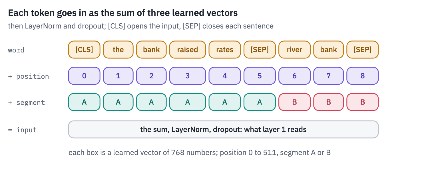
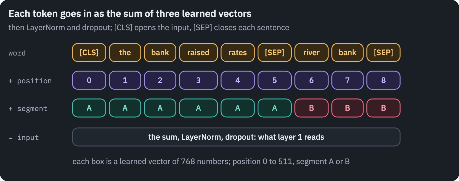
This is the encoder of the 2017 Transformer with two differences you will see in the code: positions are learned vectors rather than sinusoids, and there is a third embedding, the segment, which says whether a token belongs to the first or the second of two sentences.
512 positions is the most BERT can read at once, a limit we will run into in section 7.
The headers of the weight file list every tensor with its shape, and the Hub serves just the headers. Summed by where they live:
metadata = get_safetensors_metadata(BERT)
tensors = {}
for file_metadata in metadata.files_metadata.values():
    for name, info in file_metadata.tensors.items():
        tensors[name] = info.shape


def part_of(name):
    if name == "bert.embeddings.word_embeddings.weight":
        return "word embeddings"
    if name.startswith("bert.embeddings."):
        return "positions, segments, norm"
    if ".attention." in name:
        return "attention, 12 layers"
    if ".intermediate." in name or ".output." in name:
        return "feed-forward, 12 layers"
    if name.startswith("bert.pooler."):
        return "pooler"
    return "pre-training heads"


parts = {}
for name, shape in tensors.items():
    parts[part_of(name)] = parts.get(part_of(name), 0) + math.prod(shape)
total = sum(parts.values())
print(f"{len(tensors)} tensors, {total:,} parameters")

fig, ax = plt.subplots(figsize=(6.4, 2.9))
names = list(parts)[::-1]
ax.barh(names, [parts[n] / 1e6 for n in names], color=COLORS["enc"])
for k, n in enumerate(names):
    label = f"{parts[n] / 1e6:.1f}M"
    ax.text(parts[n] / 1e6 + 0.8, k, label, va="center", color=COLORS["muted"])
ax.set_title("Where BERT-base's parameters live")
ax.set_xlabel("millions of parameters")
ax.grid(axis="y", visible=False)
plt.show()
206 tensors, 110,106,428 parameters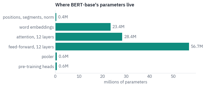
One matrix stands out. The word embeddings, one 768-number row for each of the 30,522 entries of the vocabulary, take a fifth of the model, as much as three of its twelve layers. That is why the multilingual BERT, which needs a vocabulary for 104 languages, is bigger than the English one with exactly the same layers.
Two names in the list are a little archaeological. Every LayerNorm stores gamma and beta rather than PyTorch’s weight and bias: Google trained BERT in TensorFlow, and the converted weights kept their names. And there is no output matrix for the masked word prediction at all.
The model predicts a word by comparing its hidden state with the very same embedding table it reads words from; the input and output vocabularies share one matrix.
3. WordPiece and what goes in
BERT reads WordPiece tokens. WordPiece builds its vocabulary like BPE in lesson 1 of the first course, by merging frequent pieces, but it picks the merge that most increases the likelihood of the training text rather than the most frequent pair, and it marks the pieces that continue a word with ##. Here are two sentences as BERT receives them:
tokenizer = AutoTokenizer.from_pretrained(BERT)
pair = tokenizer("The bank raised its rates.", "We sat on the river bank, unbothered.")
tokens = tokenizer.convert_ids_to_tokens(pair["input_ids"])
token_chips([tokens], ids=[pair["input_ids"]], mark_spaces=False, max_width=620,
            strong=lambda row, col, token: token in ("[CLS]", "[SEP]"))
print("segments:", pair["token_type_ids"])
segments: [0, 0, 0, 0, 0, 0, 0, 0, 1, 1, 1, 1, 1, 1, 1, 1, 1, 1, 1, 1]
[CLS] opens every input; its final hidden state is meant to summarise the whole input for classification. [SEP] closes each sentence.
The segment ids, 0 for the first sentence and 1 for the second, were needed for BERT’s second training game, next sentence prediction: half of the training pairs were real consecutive sentences and half were random ones, and BERT had to tell which.
The game turned out to be nearly useless, and the next lesson’s RoBERTa dropped it. Unbothered was not frequent enough to get a token of its own and is spelled out in pieces: nothing is ever out of vocabulary.
This is the uncased BERT: its tokenizer lowercases everything and strips accents before splitting. Google also released a cased one. The difference matters more than it sounds:
cased_tokenizer = AutoTokenizer.from_pretrained("google-bert/bert-base-cased")
name = "Eufemia Gordillo-Pagès"
token_chips([tokenizer.tokenize(name), cased_tokenizer.tokenize(name)],
            labels=["uncased", "cased"], max_width=620)


Lowercasing helps a model that reads queries typed in a hurry. It hurts a model that must find names: the capital letters are gone, and stripping the accent turns the end of a Spanish surname into the English word pages. In section 7 we will look for names, and switch to the cased BERT.
Each token becomes the sum of three learned vectors, its word, its position and its segment:
4. BERT in PyTorch
The embeddings first: three tables, added, normalised. Dropout is part of the model; it is active while training and does nothing in eval() mode.
class Embeddings(nn.Module):
    def __init__(self, config):
        super().__init__()
        d = config["hidden_size"]
        self.words = nn.Embedding(config["vocab_size"], d)
        self.positions = nn.Embedding(config["max_position_embeddings"], d)
        self.segments = nn.Embedding(config["type_vocab_size"], d)
        self.norm = nn.LayerNorm(d, eps=config["layer_norm_eps"])
        self.dropout = nn.Dropout(config["hidden_dropout_prob"])

    def forward(self, ids, segments):
        positions = torch.arange(ids.shape[1], device=ids.device)
        x = self.words(ids) + self.positions(positions) + self.segments(segments)
        return self.dropout(self.norm(x))
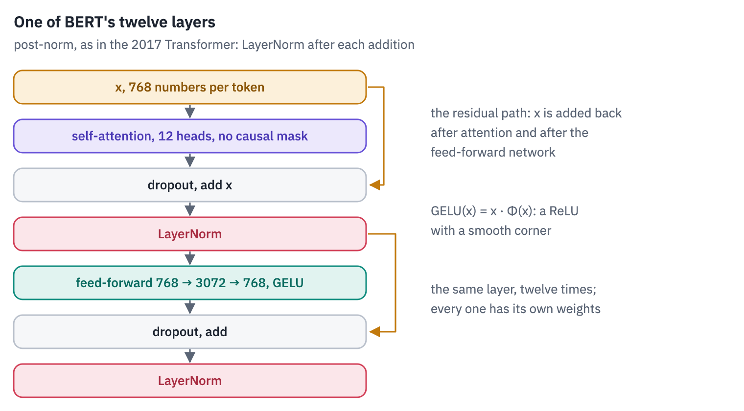
Self-attention is the one from the first course, with one difference that is the whole point: there is no causal mask. Every token attends to every other token. The only mask hides padding, the filler that makes the sentences of a batch equally long.
padding is True at those positions, and their scores become \(-\infty\) before the softmax, so they get zero weight. The layer can also hand back its attention weights, which we will look at in section 6.
class SelfAttention(nn.Module):
    def __init__(self, config):
        super().__init__()
        d = config["hidden_size"]
        self.heads = config["num_attention_heads"]
        self.q = nn.Linear(d, d)
        self.k = nn.Linear(d, d)
        self.v = nn.Linear(d, d)
        self.out = nn.Linear(d, d)
        self.dropout = nn.Dropout(config["attention_probs_dropout_prob"])

    def split(self, x):
        batch, length, d = x.shape
        return x.view(batch, length, self.heads, d // self.heads).transpose(1, 2)

    def forward(self, x, padding, keep_weights=False):
        q, k, v = self.split(self.q(x)), self.split(self.k(x)), self.split(self.v(x))
        scores = q @ k.transpose(-2, -1) / math.sqrt(q.shape[-1])
        scores = scores.masked_fill(padding[:, None, None, :], float("-inf"))
        weights = scores.softmax(dim=-1)
        y = self.dropout(weights) @ v
        y = y.transpose(1, 2).reshape(x.shape)
        return self.out(y), (weights if keep_weights else None)
A layer of BERT normalises after adding the residual, as the 2017 Transformer did; the next lessons’ models moved the norm before. The feed-forward part uses GELU, \(\text{GELU}(x) = x\,\Phi(x)\), where \(\Phi\) is the standard normal distribution function: a ReLU whose corner is smoothed, so that small negative inputs pass a little.
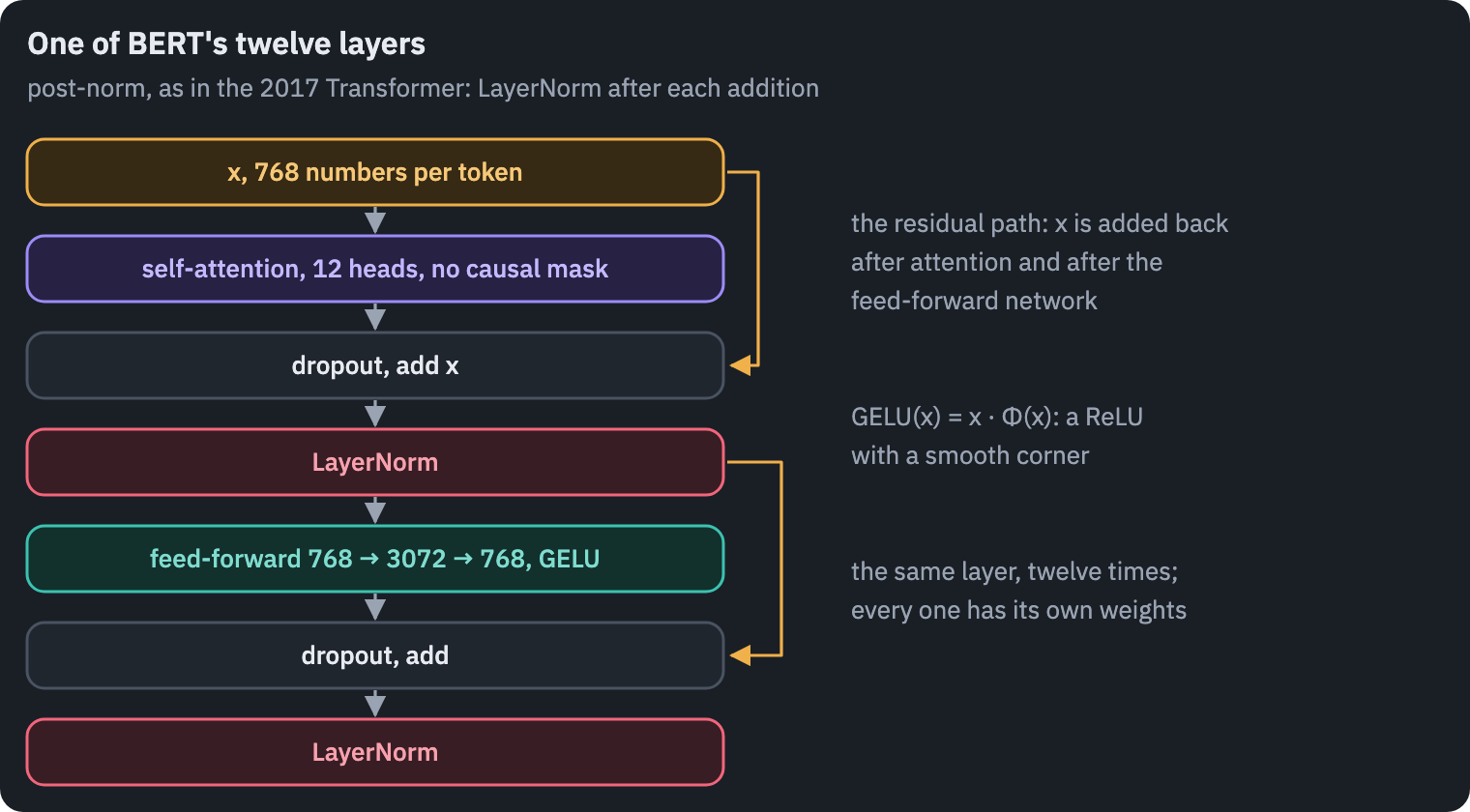
class Layer(nn.Module):
    def __init__(self, config):
        super().__init__()
        d, eps = config["hidden_size"], config["layer_norm_eps"]
        self.attention = SelfAttention(config)
        self.norm1 = nn.LayerNorm(d, eps=eps)
        self.up = nn.Linear(d, config["intermediate_size"])
        self.down = nn.Linear(config["intermediate_size"], d)
        self.norm2 = nn.LayerNorm(d, eps=eps)
        self.dropout = nn.Dropout(config["hidden_dropout_prob"])

    def forward(self, x, padding, keep_weights=False):
        a, weights = self.attention(x, padding, keep_weights)
        x = self.norm1(x + self.dropout(a))
        f = self.down(F.gelu(self.up(x)))
        x = self.norm2(x + self.dropout(f))
        return x, weights


class Bert(nn.Module):
    def __init__(self, config):
        super().__init__()
        self.embeddings = Embeddings(config)
        n_layers = config["num_hidden_layers"]
        self.layers = nn.ModuleList(Layer(config) for _ in range(n_layers))

    def forward(self, ids, segments, padding, keep_weights=False):
        x = self.embeddings(ids, segments)
        attention = []
        for layer in self.layers:
            x, weights = layer(x, padding, keep_weights)
            attention.append(weights)
        return x, attention
The head that predicts hidden words is small: a dense layer, GELU, LayerNorm, and then a dot product of the result with every row of the word embedding table, plus a bias per word. The table is not copied; the head holds the same nn.Embedding the model reads with, so training the head trains the embeddings too.
class MaskedLMHead(nn.Module):
    def __init__(self, config, words):
        super().__init__()
        d = config["hidden_size"]
        self.dense = nn.Linear(d, d)
        self.norm = nn.LayerNorm(d, eps=config["layer_norm_eps"])
        self.words = words  # the input embeddings, shared
        self.bias = nn.Parameter(torch.zeros(config["vocab_size"]))

    def forward(self, h):
        h = self.norm(F.gelu(self.dense(h)))
        return h @ self.words.weight.T + self.bias


class MaskedLM(nn.Module):
    def __init__(self, config):
        super().__init__()
        self.bert = Bert(config)
        self.head = MaskedLMHead(config, self.bert.embeddings.words)

    def forward(self, ids, segments, padding):
        h, _ = self.bert(ids, segments, padding)
        return self.head(h)
Now the transplant. Our names differ from Google’s, so we write down which of their tensors goes where, load the file and let load_state_dict refuse anything missing or left over:
def google_names(config):
    names = {
        "bert.embeddings.words.weight": "bert.embeddings.word_embeddings.weight",
        "bert.embeddings.positions.weight": "bert.embeddings.position_embeddings.weight",
        "bert.embeddings.segments.weight": "bert.embeddings.token_type_embeddings.weight",
        "bert.embeddings.norm.weight": "bert.embeddings.LayerNorm.gamma",
        "bert.embeddings.norm.bias": "bert.embeddings.LayerNorm.beta",
        "head.dense.weight": "cls.predictions.transform.dense.weight",
        "head.dense.bias": "cls.predictions.transform.dense.bias",
        "head.norm.weight": "cls.predictions.transform.LayerNorm.gamma",
        "head.norm.bias": "cls.predictions.transform.LayerNorm.beta",
        "head.words.weight": "bert.embeddings.word_embeddings.weight",  # the shared table
        "head.bias": "cls.predictions.bias",
    }
    layer_parts = {
        "attention.q": "attention.self.query", "attention.k": "attention.self.key",
        "attention.v": "attention.self.value", "attention.out": "attention.output.dense",
        "up": "intermediate.dense", "down": "output.dense",
    }
    norms = {"norm1": "attention.output.LayerNorm", "norm2": "output.LayerNorm"}
    for i in range(config["num_hidden_layers"]):
        ours, theirs = f"bert.layers.{i}.", f"bert.encoder.layer.{i}."
        for a, b in layer_parts.items():
            names[ours + a + ".weight"] = theirs + b + ".weight"
            names[ours + a + ".bias"] = theirs + b + ".bias"
        for a, b in norms.items():
            names[ours + a + ".weight"] = theirs + b + ".gamma"
            names[ours + a + ".bias"] = theirs + b + ".beta"
    return names


def load_masked_lm(repo):
    with open(hf_hub_download(repo, "config.json")) as f:
        config = json.load(f)
    weights = load_file(hf_hub_download(repo, "model.safetensors"))
    model = MaskedLM(config)
    state = {ours: weights[theirs] for ours, theirs in google_names(config).items()}
    model.load_state_dict(state, strict=True)
    return model, config


mlm, config = load_masked_lm(BERT)
mlm = mlm.to(device).eval()
print(f"loaded {sum(p.numel() for p in mlm.parameters()):,} parameters into our model")
loaded 109,514,298 parameters into our modelTwo of Google’s tensors were not used: the pooler and the next-sentence head, which only the abandoned second game needs. Does our model compute what Google’s does?
Hugging Face’s BertForMaskedLM is the reference implementation. Both models get the same two sentences; we compare the hidden states of the last layer and the scores of every word of the vocabulary at every position:
reference = BertForMaskedLM.from_pretrained(BERT).to(device).eval()
check = tokenizer(["The bank raised its rates.", "We sat on the river bank, unbothered."],
                  padding=True, return_tensors="pt").to(device)
padding = check["attention_mask"] == 0
with torch.no_grad():
    theirs = reference(**check, output_hidden_states=True)
    hidden, _ = mlm.bert(check["input_ids"], check["token_type_ids"], padding)
    logits = mlm.head(hidden)

real = ~padding  # padded positions hold numbers nobody reads
hidden_gap = (hidden - theirs.hidden_states[-1])[real].abs().max().item()
logits_gap = (logits - theirs.logits)[real].abs().max().item()
print(f"largest difference, hidden states: {hidden_gap:.1e}")
print(f"largest difference, word scores:   {logits_gap:.1e}")
assert hidden_gap < 1e-3 and logits_gap < 1e-2
del reference
largest difference, hidden states: 8.4e-05
largest difference, word scores:   1.1e-04
The differences are rounding: the two implementations add the same numbers in a different order. Our sixty lines are BERT.
5. Filling in the blanks
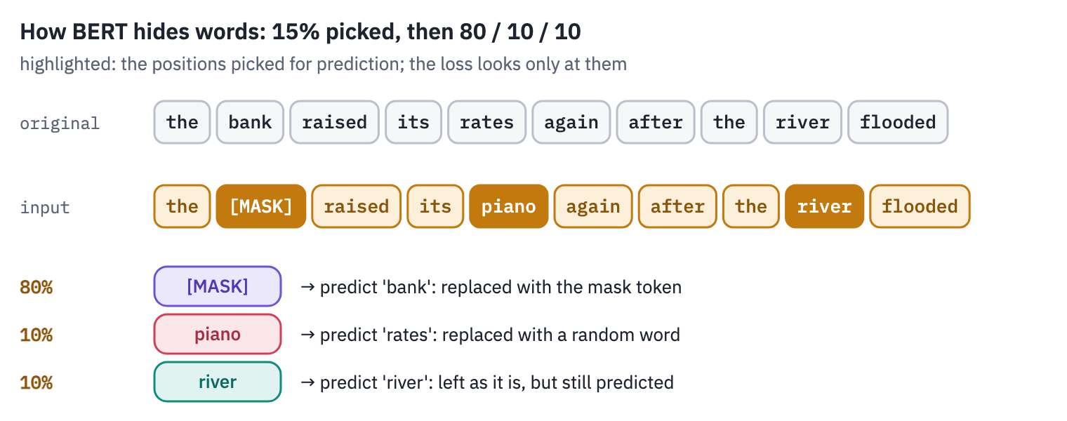
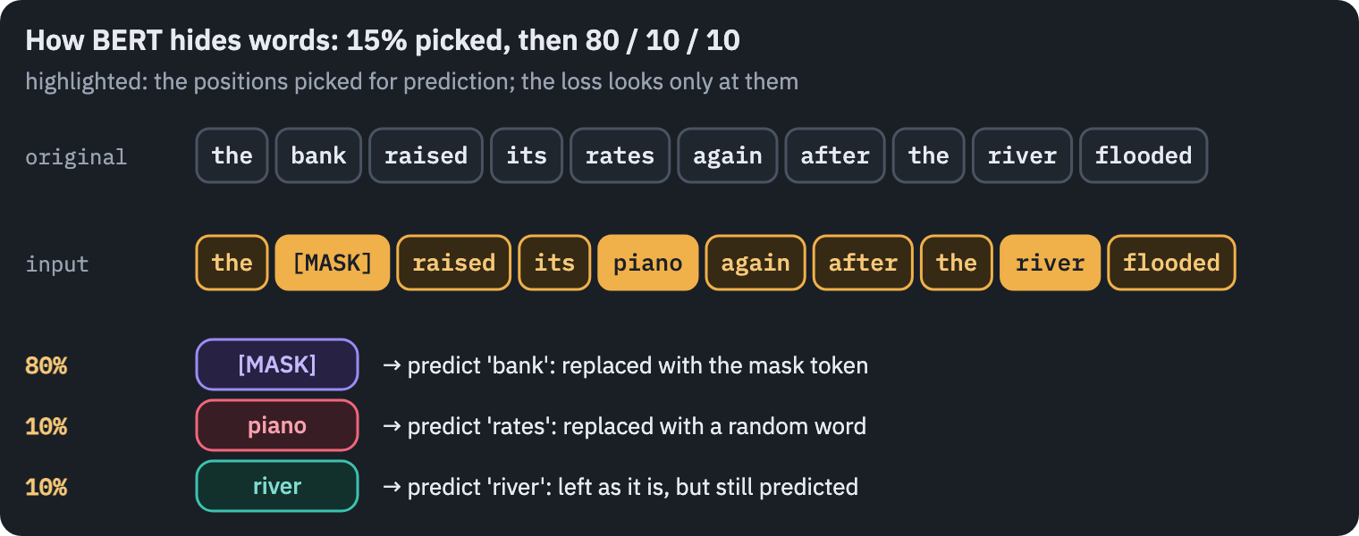
Pre-training picks 15% of the tokens of every sequence at random, never [CLS] or [SEP], and asks the model to restore them. If every picked token became [MASK], the model would learn something slightly wrong: that only [MASK] positions need predicting, while in fine-tuning [MASK] never appears.
The paper calls this “a mismatch between pre-training and fine-tuning” and softens it with a rule that every BERT-like model has copied since: of the picked tokens, 80% become [MASK], 10% become a random token, and 10% stay as they are.
The model never knows which tokens are real, so it has to keep a good guess for every position.
def mask_tokens(ids, special, generator, rate=0.15):
    chosen = (torch.rand(ids.shape, generator=generator) < rate) & ~special
    labels = ids.clone()
    labels[~chosen] = -100  # the loss ignores positions that weren't picked
    roll = torch.rand(ids.shape, generator=generator)
    masked = ids.clone()
    masked[chosen & (roll < 0.8)] = tokenizer.mask_token_id
    swap = chosen & (roll >= 0.8) & (roll < 0.9)
    random_ids = torch.randint(len(tokenizer), ids.shape, generator=generator)
    masked[swap] = random_ids[swap]
    return masked, labels


TEXT = ("In October 2019 Google changed the way its search engine reads queries. The old "
        "system treated the little word to as noise and returned results about American "
        "citizens travelling to Brazil, which is the other way around. The new one "
        "understood that the traveller goes from Brazil to the United States.")
encoded = tokenizer(TEXT, return_tensors="pt", return_special_tokens_mask=True)
ids = encoded["input_ids"]
special = encoded["special_tokens_mask"].bool()
generator = torch.Generator().manual_seed(7)
masked, labels = mask_tokens(ids, special, generator)
before = tokenizer.convert_ids_to_tokens(ids[0])
after = tokenizer.convert_ids_to_tokens(masked[0])
token_chips([before, after], labels=["original", "input"], max_width=640,
            strong=lambda row, col, token: bool(labels[0, col] != -100))
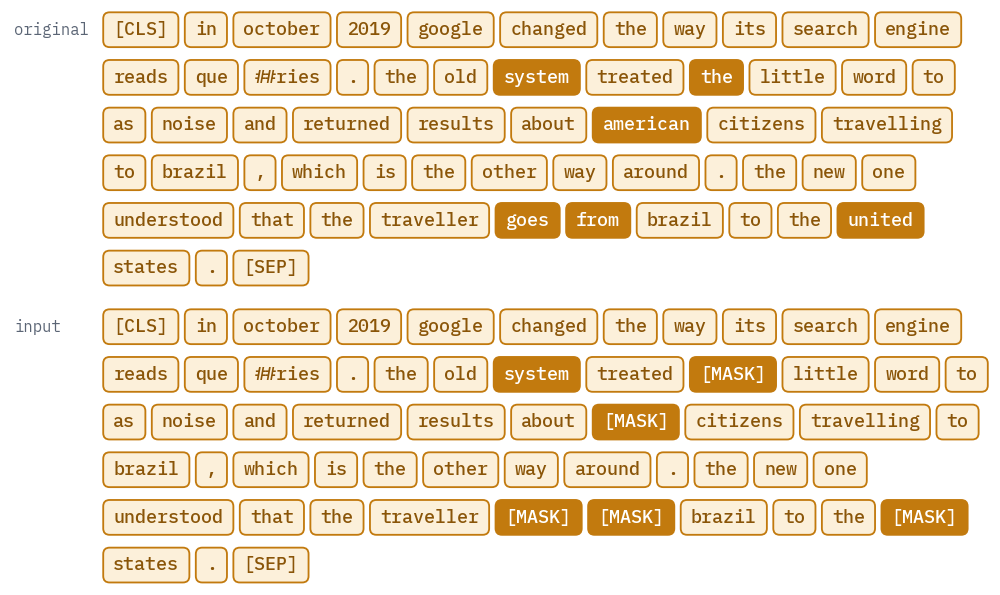
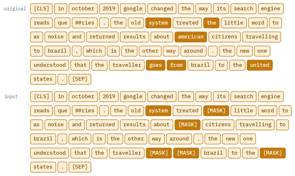
The highlighted positions are the ones the loss looks at: some became [MASK], and with this many tokens you may also see a word replaced by a random one, or a picked word left alone. Over many sequences the shares settle at what the rule says:
many = ids.repeat(4000, 1)
masked_many, labels_many = mask_tokens(many, special.repeat(4000, 1), generator)
picked = labels_many != -100
print(f"picked for prediction: {picked.float().mean():.1%} of all tokens")
became_mask = (masked_many[picked] == tokenizer.mask_token_id).float().mean()
unchanged = (masked_many[picked] == many[picked]).float().mean()
print(f"  became [MASK]:   {became_mask:.1%}")
print(f"  left unchanged:  {unchanged:.1%}")
print(f"  became another:  {1 - became_mask - unchanged:.1%}")
picked for prediction: 14.4% of all tokens
  became [MASK]:   79.9%
  left unchanged:  10.3%
  became another:  9.9%
A random replacement can occasionally draw the original word back, so “left unchanged” comes out a hair above 10%. Google’s own data generator picked exactly 15% of each sequence rather than tossing a coin per token; the coin is what most libraries do today, and it makes no difference that anyone has measured.
The share picked is a little under 15% because [CLS] and [SEP] are never picked.
The loss is cross-entropy over the vocabulary at the picked positions. On a text BERT has never seen, the first paragraph of this lesson, here is what four days of pre-training bought, against the same network as it was before training: weights drawn at random with a standard deviation of 0.02, the way BERT’s were initialised.
def masked_lm_loss(model, ids, special, repeats=20):
    generator = torch.Generator().manual_seed(0)
    losses = []
    for _ in range(repeats):
        masked, labels = mask_tokens(ids, special, generator)
        segments = torch.zeros_like(masked)
        padding = torch.zeros_like(masked, dtype=torch.bool)
        with torch.no_grad():
            logits = model(masked.to(device), segments.to(device), padding.to(device))
        loss = F.cross_entropy(logits.view(-1, logits.shape[-1]).float(),
                               labels.view(-1).to(device), ignore_index=-100)
        losses.append(loss.item())
    return sum(losses) / len(losses)


def init_like_bert(module):  # how BERT started: small random weights
    if isinstance(module, (nn.Linear, nn.Embedding)):
        nn.init.normal_(module.weight, std=0.02)
    if isinstance(module, nn.Linear) and module.bias is not None:
        nn.init.zeros_(module.bias)
    if isinstance(module, nn.LayerNorm):
        nn.init.ones_(module.weight)
        nn.init.zeros_(module.bias)


untrained = MaskedLM(config)
untrained.apply(init_like_bert)
untrained = untrained.to(device).eval()
print(f"random weights:  loss {masked_lm_loss(untrained, ids, special):.2f}")
print(f"BERT's weights:  loss {masked_lm_loss(mlm, ids, special):.2f}")
print(f"guessing uniformly among {len(tokenizer):,} tokens: {math.log(len(tokenizer)):.2f}")
del untrained
random weights:  loss 10.33
BERT's weights:  loss 3.00
guessing uniformly among 30,522 tokens: 10.33
A loss of \(L\) means the model gives the right word a probability of \(e^{-L}\) on average, in the geometric sense. The untrained network is no better than picking from the dictionary blindfolded. BERT gives the hidden word a sizeable probability most of the time, on a text written years after it was trained.
That makes BERT a strange kind of oracle: ask it to fill a blank, and you see what it absorbed from books and Wikipedia. Petroni and colleagues used exactly this to show that BERT holds “relational knowledge competitive with traditional NLP methods”[6]. Our own probes:
def fill_mask(text, k=3):
    batch = tokenizer(text, return_tensors="pt").to(device)
    padding = batch["attention_mask"] == 0
    with torch.no_grad():
        logits = mlm(batch["input_ids"], batch["token_type_ids"], padding)
    where = (batch["input_ids"][0] == tokenizer.mask_token_id).nonzero()[0, 0]
    probs = logits[0, where].float().softmax(dim=-1)
    top = probs.topk(k)
    words = tokenizer.convert_ids_to_tokens(top.indices.tolist())
    return ", ".join(f"{w} {p:.0%}" for w, p in zip(words, top.values.tolist()))


PROBES = [
    ("a fact", "The capital of Portugal is [MASK]."),
    ("a fact", "Dante was born in [MASK]."),
    ("common sense", "You cut bread with a [MASK]."),
    ("grammar", "The keys to the old cabinet [MASK] on the kitchen table."),
    ("grammar", "The key to the old cabinets [MASK] on the kitchen table."),
    ("negation", "A robin is a [MASK]."),
    ("negation", "A robin is not a [MASK]."),
    ("negation", "Birds can [MASK]."),
    ("negation", "Birds cannot [MASK]."),
]
table(pd.DataFrame({"probe": [kind for kind, _ in PROBES],
                    "sentence": [text for _, text in PROBES],
                    "BERT's top three": [fill_mask(text) for _, text in PROBES]}))
| probe | sentence | BERT's top three |
|---|---|---|
| a fact | The capital of Portugal is [MASK]. | lisbon 73%, porto 20%, madeira 0% |
| a fact | Dante was born in [MASK]. | rome 5%, paris 4%, london 2% |
| common sense | You cut bread with a [MASK]. | knife 72%, stick 8%, fork 4% |
| grammar | The keys to the old cabinet [MASK] on the kitchen table. | were 52%, sat 17%, lay 12% |
| grammar | The key to the old cabinets [MASK] on the kitchen table. | was 41%, lay 18%, sat 18% |
| negation | A robin is a [MASK]. | robin 38%, bird 32%, pigeon 1% |
| negation | A robin is not a [MASK]. | robin 57%, bird 10%, pigeon 1% |
| negation | Birds can [MASK]. | fly 19%, sing 9%, breed 8% |
| negation | Birds cannot [MASK]. | fly 37%, sing 10%, escape 3% |
The knowledge is patchy in a revealing way. BERT is sure about Lisbon and the knife, and has no idea where Dante was born: a fact that is stated less often in so many words.
The grammar is right, and it is the impressive row. The verb agrees with keys or key, the subject, and not with cabinet or cabinets, the noun right next to it, so the model must know which word the verb belongs to.
Negation is where it breaks. To BERT a robin is above all a robin, and it is more sure that birds cannot fly than that they can.
Kassner and Schütze found this across models and put it in the title of their paper, “Birds Can Talk, But Cannot Fly”: pre-trained models “do not distinguish between negated (‘Birds cannot [MASK]’) and non-negated (‘Birds can [MASK]’) cloze questions”[7].
Filling a blank rewards knowing which words go together, and birds and fly go together whether or not there is a not between them.
The same oracle shows what else came with the books. Give BERT a sentence about a person with a job and ask for the pronoun:
JOBS = ["nurse", "receptionist", "secretary", "librarian", "hairdresser", "teacher",
        "cashier", "baker", "accountant", "doctor", "lawyer", "scientist", "programmer",
        "engineer", "pilot", "mechanic", "carpenter", "surgeon", "firefighter", "farmer"]
he, she = tokenizer.convert_tokens_to_ids(["he", "she"])
shares = {}
for job in JOBS:
    sentence = f"the {job} said that [MASK] would be late."
    batch = tokenizer(sentence, return_tensors="pt").to(device)
    padding = batch["attention_mask"] == 0
    with torch.no_grad():
        logits = mlm(batch["input_ids"], batch["token_type_ids"], padding)
    where = (batch["input_ids"][0] == tokenizer.mask_token_id).nonzero()[0, 0]
    probs = logits[0, where].float().softmax(dim=-1)
    shares[job] = (probs[she] / (probs[he] + probs[she])).item()

order = sorted(shares, key=shares.get)
fig, ax = plt.subplots(figsize=(6.4, 5.2))
ax.barh(order, [shares[j] for j in order], color=COLORS["att"])
ax.axvline(0.5, color=COLORS["muted"], linewidth=1, linestyle="--")
ax.set_xlim(0, 1)
ax.set_title("“The ___ said that [MASK] would be late”: she or he?")
ax.set_xlabel("P(she) / (P(she) + P(he))")
ax.grid(axis="y", visible=False)
plt.show()
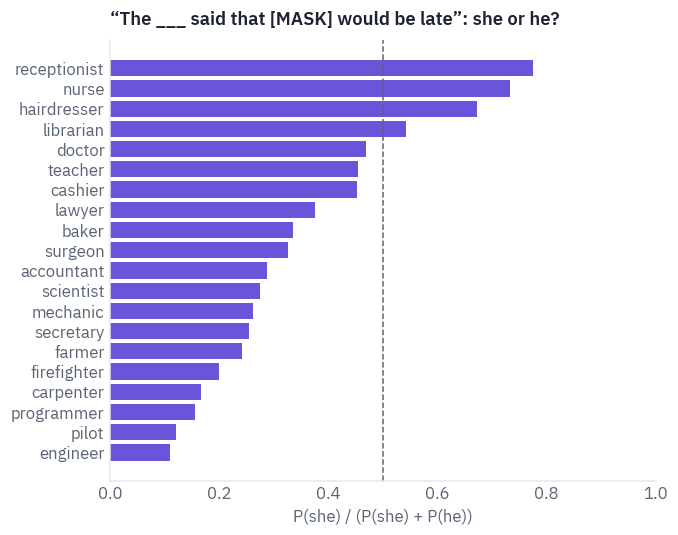
Nothing in the sentence says anything about the person’s gender, and the dashed line is where a model with no opinion would put every job. BERT has opinions.
Receptionists, nurses and hairdressers are she; engineers, pilots and programmers are he; and most jobs, the doctor and the teacher among them, lean he. These are the statistics of its training text.
Kurita and colleagues measured them this way, with templates and the masked word’s probabilities, and showed that such associations carry into the models fine-tuned from BERT [8]. It is worth remembering when a BERT-based classifier screens CVs.
6. What the heads look at
BERT-base has 144 attention heads, 12 in each of 12 layers, and nobody told any of them what to do.
Clark and colleagues looked at all of them and found heads attending “to delimiter tokens, specific positional offsets, or broadly attending over the whole sentence”, and some that “correspond well to linguistic notions of syntax and coreference”[9].
Our model hands back its attention weights, so we can measure the same thing on a few hundred sentences of Wikipedia: for every head, how much of its attention goes to [CLS], to [SEP], to the previous token and to the next one, averaged over all real tokens.
wiki = load_dataset("Salesforce/wikitext", "wikitext-2-raw-v1", split="test")
sentences = [line.strip() for line in wiki["text"] if len(line.strip()) > 200]
sentences = sentences[:32 if SMOKE else 320]

layers, heads = config["num_hidden_layers"], config["num_attention_heads"]
TARGETS = ["[CLS]", "[SEP]", "previous", "next"]
totals = {name: torch.zeros(layers, heads) for name in TARGETS}
count = 0
for start in range(0, len(sentences), 32):
    batch = tokenizer(sentences[start:start + 32], padding=True, truncation=True,
                      max_length=128, return_tensors="pt").to(device)
    padding = batch["attention_mask"] == 0
    with torch.no_grad():
        _, attention = mlm.bert(batch["input_ids"], batch["token_type_ids"], padding,
                                keep_weights=True)
    weights = torch.stack(attention, dim=1).float()  # batch, layer, head, query, key
    real = (~padding).float()
    is_sep = (batch["input_ids"] == tokenizer.sep_token_id).float()
    to_cls = weights[..., 0]
    to_sep = (weights * is_sep[:, None, None, None, :]).sum(-1)
    to_prev = torch.diagonal(weights, offset=-1, dim1=-2, dim2=-1)
    to_next = torch.diagonal(weights, offset=1, dim1=-2, dim2=-1)
    totals["[CLS]"] += (to_cls * real[:, None, None, :]).sum((0, 3)).cpu()
    totals["[SEP]"] += (to_sep * real[:, None, None, :]).sum((0, 3)).cpu()
    totals["previous"] += (to_prev * real[:, None, None, 1:]).sum((0, 3)).cpu()
    totals["next"] += (to_next * real[:, None, None, :-1]).sum((0, 3)).cpu()
    count += real.sum().item()
shares_by_head = {name: (value / count).numpy() for name, value in totals.items()}

fig, axes = plt.subplots(1, 4, figsize=(12, 3.6))
for ax, (name, values) in zip(axes, shares_by_head.items()):
    heatmap(values, rows=range(1, layers + 1), cols=range(1, heads + 1), ax=ax,
            vmin=0, vmax=1, cell=0.22, title=f"to {name}",
            xlabel="head", ylabel="layer" if ax is axes[0] else None)
plt.tight_layout()
plt.show()
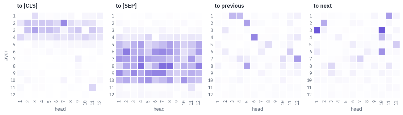
The layers divide the work. In layers 2 to 4 attention gathers on [CLS]; in layers 5 to 10 almost every head sends much of it to [SEP], a token that carries no information about any particular word; the last two layers spread out again.
Clark and colleagues suggested that a head with nothing useful to do in a given context parks its attention on [SEP], a no-op: softmax has to send the weight somewhere.
The first layers also have heads that look almost only one token back or one token ahead, which is how a model with no built-in notion of order puts neighbouring words together. Here is the most devoted previous-token head on one sentence:
layer, head = np.unravel_index(shares_by_head["previous"].argmax(), (layers, heads))
example = "The traveller from Brazil needs a visa to enter the United States."
batch = tokenizer(example, return_tensors="pt").to(device)
with torch.no_grad():
    _, attention = mlm.bert(batch["input_ids"], batch["token_type_ids"],
                            batch["attention_mask"] == 0, keep_weights=True)
words = tokenizer.convert_ids_to_tokens(batch["input_ids"][0])
heatmap(attention[layer][0, head].float().cpu().numpy(), rows=words, cols=words, cell=0.28,
        title=f"Layer {layer + 1}, head {head + 1}: where each word looks",
        xlabel="attends to", ylabel="word")
plt.show()
print(f"on average this head puts {shares_by_head['previous'][layer, head]:.0%} "
      "of its attention on the previous token")
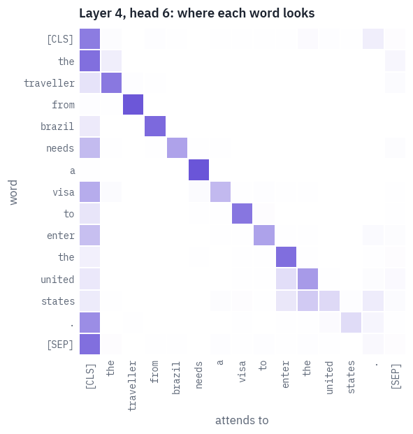
on average this head puts 71% of its attention on the previous tokenHeads like this one are why reading “attention maps” as explanations is risky. Most of what a head does is plumbing: moving information to where the next layer can use it. The linguistically interesting heads exist, but they are a minority, and a head that looks at a word doesn’t mean the model uses what it found.
7. A job for BERT: personal data in financial documents
Banks, insurers and their software vendors move a lot of text around: support tickets, loan applications, SWIFT messages, contracts. Before such text goes into a log, a search index, a test environment or a prompt for some external model, the personal data in it has to be found and masked: names, addresses, account numbers, phone numbers.
Regular expressions find the things with a fixed shape. Names and addresses have no fixed shape, and that is a classic job for an encoder: named entity recognition, a label for every token.
Real documents full of real personal data are, for good reasons, not something anyone publishes. Gretel’s dataset is synthetic: about 56,000 documents of 60 kinds, in seven languages, written by a language model and annotated with the character spans of 29 kinds of personal data [10]. We take the English ones.
pii = load_dataset("gretelai/synthetic_pii_finance_multilingual")
english = pii.filter(lambda row: row["language"] == "English")
train_rows, test_rows = english["train"], english["test"]
if SMOKE:
    train_rows, test_rows = train_rows.select(range(96)), test_rows.select(range(24))
print(f"{len(train_rows):,} documents to train on, {len(test_rows):,} to test on")
print(f"{len(set(train_rows['document_type']))} kinds, e.g.:",
      ", ".join(sorted(set(train_rows["document_type"]))[:8]))
25,948 documents to train on, 2,962 to test on
60 kinds, e.g.: Annual Report, Audit Report, BAI Format, Bank Statement, Bill of Lading, Business Plan, CSV, Compliance Certificate
The 29 kinds of the annotation are more than we need to see. We fold them into twelve groups, which is roughly how a masking policy would treat them: a first name and a full name are both a person, an IBAN and a routing number are both bank details.
GROUPS = {
    "name": "PERSON", "first_name": "PERSON", "last_name": "PERSON",
    "company": "COMPANY",
    "street_address": "ADDRESS",
    "local_latlng": "LOCATION",
    "date": "DATE", "date_of_birth": "DATE", "date_time": "DATE", "time": "DATE",
    "email": "EMAIL",
    "phone_number": "PHONE",
    "iban": "BANK", "bban": "BANK", "swift_bic_code": "BANK", "bank_routing_number": "BANK",
    "credit_card_number": "CARD", "credit_card_security_code": "CARD",
    "ssn": "GOV_ID", "passport_number": "GOV_ID", "driver_license_number": "GOV_ID",
    "customer_id": "ACCOUNT", "employee_id": "ACCOUNT", "account_pin": "ACCOUNT",
    "ipv4": "DIGITAL", "ipv6": "DIGITAL", "user_name": "DIGITAL", "password": "DIGITAL",
    "api_key": "DIGITAL",
}
KINDS = sorted(set(GROUPS.values()))


def gold_spans(row):
    spans = []
    for span in json.loads(row["pii_spans"]):
        spans.append((span["start"], span["end"], GROUPS[span["label"]]))
    return spans


counts = {kind: 0 for kind in KINDS}
for row in train_rows:
    for _, _, kind in gold_spans(row):
        counts[kind] += 1
order = sorted(KINDS, key=counts.get)
fig, ax = plt.subplots(figsize=(6.4, 3.6))
ax.barh(order, [counts[k] for k in order], color=COLORS["data"])
ax.set_xscale("log")
ax.set_title("Annotated spans in the training documents, by group")
ax.set_xlabel("spans (log scale)")
ax.grid(axis="y", visible=False)
plt.show()
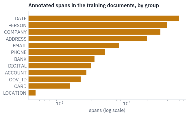
Dates, people and companies are everywhere; GPS coordinates and card numbers are rare. A model will learn the common groups easily and the rare ones from a few hundred examples each. Here is one document with its annotation:
SHADES = {"PERSON": "#D23F57", "COMPANY": "#6A55D8", "ADDRESS": "#0F8C7E",
"DATE": "#C27A0E"}
def highlight(text, spans):
pieces, last = [], 0
for start, end, kind in sorted(spans):
color = SHADES.get(kind, "#5B6575")
pieces.append(text[last:start].replace("<", "<"))
pieces.append(f'<span style="background:{color}2e;border-bottom:2px solid {color};'
f'padding:0 2px">{text[start:end]}<sub style="color:{color};'
f'font-size:0.7em"> {kind}</sub></span>')
last = end
pieces.append(text[last:].replace("<", "<"))
body = "".join(pieces)
style = "white-space:pre-wrap;font-size:0.85em;line-height:1.55"
return HTML(f'<div style="{style}">{body}</div>')
sample = train_rows[3]
print(sample["document_type"])
sample_spans = [s for s in gold_spans(sample) if s[1] <= 900]
display(highlight(sample["generated_text"][:900], sample_spans))
Health Insurance Claim FormSynthetic data has its own quirks, and this document shows two. The template line “Provider Address: [Treating Dentist’s Address]” is a placeholder the generator forgot to fill, and the annotator, also a model, marked it as an address. And a policy number is labelled as a bank account number.
A model trained on such labels will learn some of their mistakes too; when we measure it, a small share of its “errors” will be the annotation’s.
The bigger problem is length. BERT reads at most 512 tokens, two of them [CLS] and [SEP]:
lengths = [len(cased_tokenizer(text, add_special_tokens=False)["input_ids"])
           for text in test_rows["generated_text"]]
longer = sum(n > 510 for n in lengths) / len(lengths)
fig, ax = plt.subplots(figsize=(6.4, 3.2))
ax.hist(lengths, bins=40, color=COLORS["data"])
ax.axvline(510, color=COLORS["dec"], linewidth=1.5)
ax.text(520, ax.get_ylim()[1] * 0.85, "BERT's limit", color=COLORS["dec"])
ax.set_title("Length of the test documents in BERT's tokens")
ax.set_xlabel("tokens")
plt.show()
print(f"{longer:.0%} of the documents don't fit in one input")
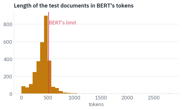
14% of the documents don't fit in one inputTruncating would silently skip whatever personal data sits past the limit, which for a masking tool is the worst kind of error.
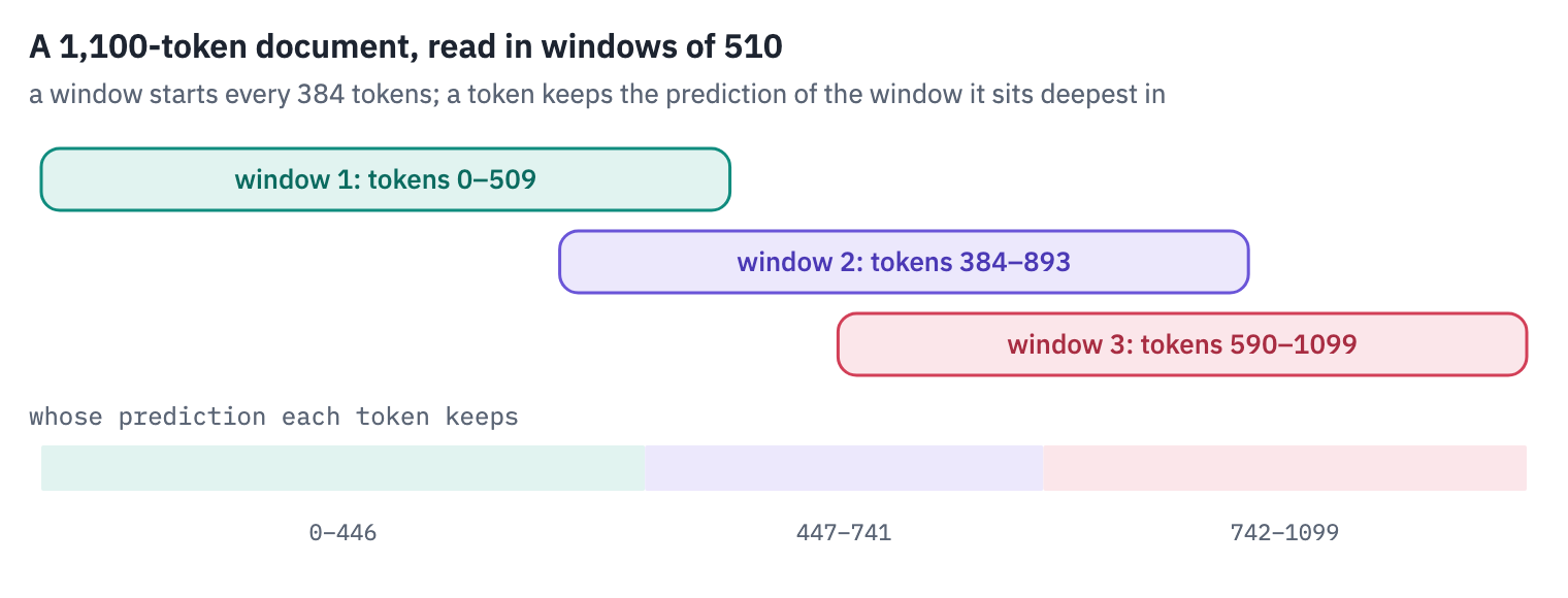
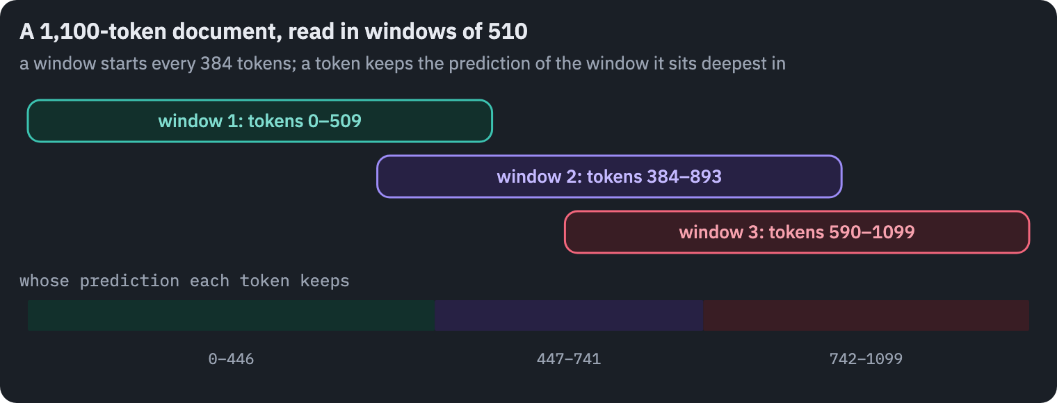
The standard fix is a sliding window: cut the document into overlapping pieces of 510 tokens, run each, and for every token keep the prediction from the window in which it sits furthest from an edge, where it had the most context on both sides.
WINDOW, STRIDE = (126, 96) if SMOKE else (510, 384)


def windows(n_tokens):
    if n_tokens <= WINDOW:
        return [(0, n_tokens)]
    starts = list(range(0, n_tokens - WINDOW + 1, STRIDE))
    if starts[-1] + WINDOW < n_tokens:
        starts.append(n_tokens - WINDOW)
    return [(start, start + WINDOW) for start in starts]


print(windows(1100))
[(0, 510), (384, 894), (590, 1100)]Labels come as character spans, and the model needs one label per token. We use the BIO scheme: B-PERSON on the first token of a name, I-PERSON on the tokens that continue it, O on everything else. The tokenizer’s offset mapping says which characters each token covers:
LABELS = ["O"] + [f"{prefix}-{kind}" for kind in KINDS for prefix in ("B", "I")]
LABEL_ID = {label: i for i, label in enumerate(LABELS)}


def encode(row):
    text = row["generated_text"]
    encoded = cased_tokenizer(text, add_special_tokens=False, return_offsets_mapping=True)
    offsets = encoded["offset_mapping"]
    tags = ["O"] * len(offsets)
    for start, end, kind in gold_spans(row):
        first = True
        for i, (a, b) in enumerate(offsets):
            if a >= start and b <= end and b > a:
                tags[i] = ("B-" if first else "I-") + kind
                first = False
    return encoded["input_ids"], offsets, tags


ids, offsets, tags = encode(sample)
shown = [(cased_tokenizer.convert_ids_to_tokens(i), t) for i, t in zip(ids[:40], tags[:40])]
token_chips([[token for token, _ in shown]], max_width=640,
            strong=lambda row, col, token: shown[col][1] != "O")
print(" ".join(tag for _, tag in shown))
O O O O O O O B-PERSON I-PERSON I-PERSON I-PERSON I-PERSON I-PERSON I-PERSON I-PERSON I-PERSON I-PERSON O O O O O O O O O O O O O O O O O O B-ADDRESS I-ADDRESS I-ADDRESS I-ADDRESS O
Each window becomes a training example: [CLS], the window’s tokens, [SEP], and labels of \(-100\) on the two special tokens so that the loss ignores them.
def examples(rows):
    out = []
    for row in rows:
        ids, _, tags = encode(row)
        for start, end in windows(len(ids)):
            window_ids = [cased_tokenizer.cls_token_id] + ids[start:end]
            window_ids += [cased_tokenizer.sep_token_id]
            window_labels = [-100] + [LABEL_ID[t] for t in tags[start:end]] + [-100]
            out.append((window_ids, window_labels))
    return out
8. Fine-tuning, and what pre-training is worth
The tagger is our Bert with one linear layer on top: 768 numbers in, one score per label out, at every position. All of BERT’s weights train along with the new layer, which is what “fine-tuning” meant in the paper.
class Tagger(nn.Module):
    def __init__(self, bert, n_labels):
        super().__init__()
        self.bert = bert
        self.dropout = nn.Dropout(0.1)
        self.classify = nn.Linear(bert.embeddings.words.embedding_dim, n_labels)

    def forward(self, ids, padding):
        h, _ = self.bert(ids, torch.zeros_like(ids), padding)
        return self.classify(self.dropout(h))


def new_tagger(pretrained):  # random weights are initialised as in section 5
    masked_lm, _ = load_masked_lm("google-bert/bert-base-cased")
    tagger = Tagger(masked_lm.bert, len(LABELS))
    if not pretrained:
        tagger.apply(init_like_bert)
    return tagger.to(device)
Training sorts the windows by length and batches neighbours together, so a batch of short windows isn’t padded to
- The rest is the recipe from the paper’s fine-tuning appendix: AdamW, a learning rate warmed up over the first tenth of the steps and then decayed linearly, a few epochs. Mixed precision keeps it fast on a T4.
def batches(data, size, shuffle):
    order = sorted(range(len(data)), key=lambda i: len(data[i][0]))
    groups = [order[i:i + size] for i in range(0, len(order), size)]
    if shuffle:
        random.shuffle(groups)
    for group in groups:
        width = max(len(data[i][0]) for i in group)
        ids = torch.full((len(group), width), cased_tokenizer.pad_token_id)
        labels = torch.full((len(group), width), -100)
        for row, i in enumerate(group):
            n = len(data[i][0])
            ids[row, :n] = torch.tensor(data[i][0])
            labels[row, :n] = torch.tensor(data[i][1])
        yield ids.to(device), labels.to(device)


def train(tagger, data, epochs=2, lr=5e-5, batch_size=16, steps=None):
    if steps:  # a fixed number of updates, however much data there is
        epochs = math.ceil(steps / math.ceil(len(data) / batch_size))
    steps = epochs * math.ceil(len(data) / batch_size)
    warmup = max(1, steps // 10)
    optimizer = torch.optim.AdamW(tagger.parameters(), lr=lr, weight_decay=0.01)
    def rate(step):  # linear warm-up, then linear decay to zero
        return min((step + 1) / warmup, max(0.0, (steps - step) / max(1, steps - warmup)))

    schedule = torch.optim.lr_scheduler.LambdaLR(optimizer, rate)
    scaler = torch.amp.GradScaler(enabled=device == "cuda")
    tagger.train()
    for _ in range(epochs):
        for ids, labels in batches(data, batch_size, shuffle=True):
            with torch.autocast(device, dtype=torch.float16, enabled=device == "cuda"):
                logits = tagger(ids, ids == cased_tokenizer.pad_token_id)
                flat = logits.view(-1, len(LABELS)).float()
                loss = F.cross_entropy(flat, labels.view(-1), ignore_index=-100)
            optimizer.zero_grad(set_to_none=True)
            scaler.scale(loss).backward()
            scaler.unscale_(optimizer)
            nn.utils.clip_grad_norm_(tagger.parameters(), 1.0)
            scaler.step(optimizer)
            scaler.update()
            schedule.step()
    return tagger.eval()
Prediction runs the windows of a document, keeps each token’s best-placed prediction, and turns runs of B- and I- labels back into character spans. Evaluation is strict: a predicted span counts only if it has the right group and exactly the right boundaries, on the token grid.
def predict(tagger, row):
    ids, offsets, _ = encode(row)
    best, depth = ["O"] * len(ids), [-1] * len(ids)
    for start, end in windows(len(ids)):
        window = [cased_tokenizer.cls_token_id] + ids[start:end]
        window = torch.tensor([window + [cased_tokenizer.sep_token_id]], device=device)
        no_padding = torch.zeros_like(window, dtype=torch.bool)
        half = torch.autocast(device, dtype=torch.float16, enabled=device == "cuda")
        with torch.no_grad(), half:
            logits = tagger(window, no_padding)
        labels = logits[0, 1:-1].argmax(-1).tolist()
        for k, label in enumerate(labels):
            i = start + k
            room = min(k, end - start - 1 - k)  # distance to the nearer edge of the window
            if room > depth[i]:
                best[i], depth[i] = LABELS[label], room
    return to_spans(best, offsets)


def to_spans(tags, offsets):
    spans, current = [], None
    for (a, b), tag in zip(offsets, tags):
        kind = tag[2:] if tag != "O" else None
        if kind and (tag.startswith("B-") or current is None or current[2] != kind):
            if current:
                spans.append(tuple(current))
            current = [a, b, kind]
        elif kind:
            current[1] = b
        elif current:
            spans.append(tuple(current))
            current = None
    if current:
        spans.append(tuple(current))
    return spans


def aligned_gold(row):
    _, offsets, tags = encode(row)
    return to_spans(tags, offsets)


def scores(predicted, gold):
    rows = []
    for kind in KINDS + ["all"]:
        hits = found = wanted = 0
        for p, g in zip(predicted, gold):
            p = {s for s in p if kind == "all" or s[2] == kind}
            g = {s for s in g if kind == "all" or s[2] == kind}
            hits, found, wanted = hits + len(p & g), found + len(p), wanted + len(g)
        precision = hits / found if found else float("nan")
        recall = hits / wanted if wanted else float("nan")
        f1 = 2 * precision * recall / (precision + recall) if hits else 0.0
        rows.append({"group": kind, "spans": wanted, "precision": precision,
                     "recall": recall, "F1": f1})
    return pd.DataFrame(rows)
First the experiment that explains why BERT mattered. The same network is fine-tuned twice on the same documents: once starting from Google’s weights, once from random ones, each with the same 300 updates of the weights. We repeat it with more and more training documents.
random.seed(SEED)
test_subset = test_rows.select(range(min(len(test_rows), 400)))
test_gold = [aligned_gold(row) for row in test_subset]
SIZES = [16] if SMOKE else [100, 400, 1600]  # CI runs on a slow CPU
curve = []
for size in SIZES:
    data = examples(train_rows.select(range(size)))
    for pretrained in (True, False):
        t0 = time.time()
        torch.manual_seed(SEED)
        tagger = train(new_tagger(pretrained), data, steps=10 if SMOKE else 300)
        predicted = [predict(tagger, row) for row in test_subset]
        f1 = scores(predicted, test_gold).set_index("group").loc["all", "F1"]
        start = "BERT's weights" if pretrained else "random"
        curve.append({"documents": size, "start": start, "F1": f1,
                      "minutes": (time.time() - t0) / 60})
        del tagger
        if device == "cuda":
            torch.cuda.empty_cache()
table(pd.DataFrame(curve))
| documents | start | F1 | minutes |
|---|---|---|---|
| 100 | BERT's weights | 0.53 | 2.33 |
| 100 | random | 0.05 | 2.42 |
| 400 | BERT's weights | 0.59 | 2.76 |
| 400 | random | 0.07 | 2.82 |
| 1,600 | BERT's weights | 0.64 | 3.12 |
| 1,600 | random | 0.08 | 3.16 |
curve_frame = pd.DataFrame(curve)
fig, ax = plt.subplots(figsize=(6.4, 3.6))
for start, color in [("BERT's weights", COLORS["enc"]), ("random", COLORS["dec"])]:
    part = curve_frame[curve_frame["start"] == start]
    ax.plot(part["documents"], part["F1"], marker="o", color=color, label=start)
ax.set_xscale("log")
ax.set_xticks(SIZES, [str(s) for s in SIZES])
ax.set_ylim(0, 1)
ax.set_title("Same network, same data: starting from pre-trained weights")
ax.set_xlabel("training documents")
ax.set_ylabel("entity F1 on the test documents")
ax.legend(frameon=False)
plt.show()
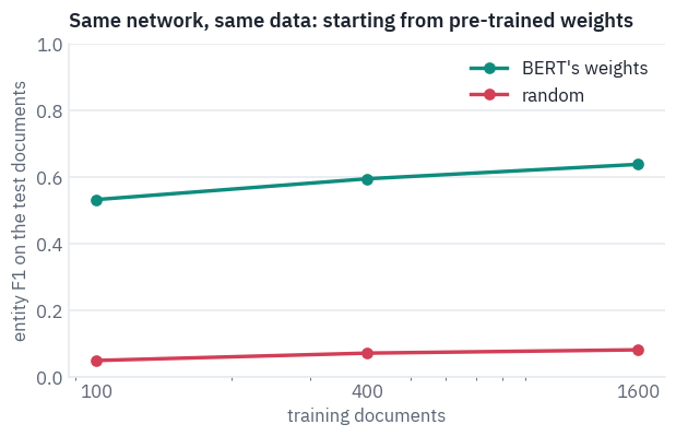
This is the chart that changed NLP in 2018. With a hundred documents the pre-trained network already gets about half of the spans exactly right.
The random one gets almost none, and sixteen times more documents barely move it: it spends its 300 updates learning that most tokens are O, while the pre-trained one starts from a model of English and only has to learn what a name or an IBAN looks like in these documents.
With far more updates and data the random network would get further; pre-training paid for those in advance. The four days of Google’s TPUs are not in the architecture, since the two networks are identical. They are in the weights.
Now the real model, on all the training documents:
train_data = examples(train_rows)
print(f"{len(train_data):,} windows from {len(train_rows):,} documents")
t0 = time.time()
torch.manual_seed(SEED)
tagger = train(new_tagger(pretrained=True), train_data, epochs=1 if SMOKE else 2)
print(f"fine-tuned in {(time.time() - t0) / 60:.1f} min")
30,142 windows from 25,948 documents
fine-tuned in 30.7 min
9. BERT against regular expressions
The fair opponent is what a careful engineer would write first: regular expressions for everything that has a shape. Emails, phone numbers, IBANs, card numbers checked with the Luhn algorithm, dates in the common formats, IP addresses, social security numbers. Names, companies and addresses get no regex, because there is no honest one to write.
MONTHS = "Jan|Feb|Mar|Apr|May|Jun|Jul|Aug|Sep|Oct|Nov|Dec"
PATTERNS = {
    "EMAIL": r"[\w.+-]+@[\w-]+(?:\.[\w-]+)+",
    "PHONE": r"(?<![\w-])(?:\+\d{1,3}[\s.-]?)?(?:\(\d{2,4}\)[\s.-]?)?\d{3}[\s.-]\d{3,4}"
             r"(?:[\s.-]\d{2,4})?(?![\w-])",
    "BANK": r"\b[A-Z]{2}\d{2}(?:\s?[A-Z0-9]{4}){2,7}(?:\s?[A-Z0-9]{1,4})?\b",
    "CARD": r"\b(?:\d[ -]?){12,18}\d\b",
    "DATE": rf"\b\d{{4}}-\d{{2}}-\d{{2}}\b|\b\d{{1,2}}/\d{{1,2}}/\d{{2,4}}\b"
            rf"|\b(?:{MONTHS})[a-z]*\.? \d{{1,2}},? \d{{4}}\b"
            rf"|\b\d{{1,2}} (?:{MONTHS})[a-z]* \d{{4}}\b"
            rf"|\b\d{{1,2}}:\d{{2}}(?::\d{{2}})?(?:\s?[AP]M)?\b",
    "DIGITAL": r"\b(?:\d{1,3}\.){3}\d{1,3}\b|\b(?:[0-9a-fA-F]{1,4}:){7}[0-9a-fA-F]{1,4}\b",
    "GOV_ID": r"\b\d{3}-\d{2}-\d{4}\b",
}


def luhn(digits):
    total = 0
    for i, d in enumerate(reversed(digits)):
        d = int(d)
        if i % 2 == 1:
            d = d * 2 - 9 if d * 2 > 9 else d * 2
        total += d
    return total % 10 == 0


def regex_spans(row):
    text = row["generated_text"]
    _, offsets, _ = encode(row)
    found = []
    for kind, pattern in PATTERNS.items():
        for match in re.finditer(pattern, text):
            if kind == "CARD" and not luhn(re.sub(r"\D", "", match.group())):
                continue
            inside = [(a, b) for a, b in offsets if a >= match.start() and b <= match.end()]
            if inside:  # the same token grid as the model's predictions
                found.append((inside[0][0], inside[-1][1], kind))
    return found


test_all = test_rows
gold_all = [aligned_gold(row) for row in test_all]
t0 = time.time()
bert_found = [predict(tagger, row) for row in test_all]
seconds = time.time() - t0
regex_found = [regex_spans(row) for row in test_all]
bert_scores = scores(bert_found, gold_all).set_index("group")
regex_scores = scores(regex_found, gold_all).set_index("group")
comparison = pd.DataFrame({"spans": bert_scores["spans"],
                           "BERT F1": bert_scores["F1"],
                           "regex F1": regex_scores["F1"].where(
                               regex_scores.index.isin(list(PATTERNS) + ["all"]))})
display(table(comparison.reset_index().fillna("—")))  # no regex for that group
print(f"BERT tagged {len(test_all):,} documents in {seconds:.0f} s, "
      f"{len(test_all) / seconds:.0f} documents a second")
| group | spans | BERT F1 | regex F1 |
|---|---|---|---|
| ACCOUNT | 281 | 0.81 | — |
| ADDRESS | 2,330 | 0.86 | — |
| BANK | 425 | 0.87 | 0.31 |
| CARD | 175 | 0.74 | 0.31 |
| COMPANY | 3,606 | 0.78 | — |
| DATE | 6,638 | 0.82 | 0.45 |
| DIGITAL | 289 | 0.76 | 0.69 |
| 844 | 0.86 | 0.93 | |
| GOV_ID | 225 | 0.85 | 0.45 |
| LOCATION | 67 | 0.59 | — |
| PERSON | 4,555 | 0.85 | — |
| PHONE | 532 | 0.90 | 0.58 |
| all | 19,967 | 0.82 | 0.30 |
BERT tagged 2,962 documents in 51 s, 58 documents a secondshown_kinds = [k for k in KINDS if bert_scores.loc[k, "spans"] > 0]
x = np.arange(len(shown_kinds))
fig, ax = plt.subplots(figsize=(8.4, 3.6))
ax.bar(x - 0.2, [bert_scores.loc[k, "F1"] for k in shown_kinds], 0.4, color=COLORS["enc"],
label="fine-tuned BERT")
regex_values = [regex_scores.loc[k, "F1"] if k in PATTERNS else 0 for k in shown_kinds]
ax.bar(x + 0.2, regex_values, 0.4, color=COLORS["data"], label="regular expressions")
ax.set_xticks(x, shown_kinds, rotation=35, ha="right")
ax.set_ylim(0, 1)
ax.set_title("Entity F1 on the test documents, by group")
ax.legend(frameon=False, loc="upper left", bbox_to_anchor=(1, 1))
plt.show()
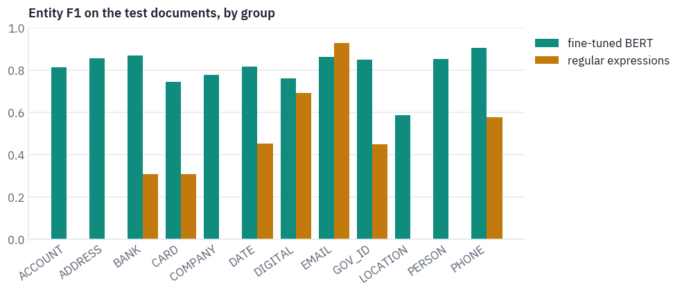
Look at emails first: there the regular expression beats the model. An email address has a strict shape, and a pattern matches it character by character, while BERT reads tokens and now and then stops a piece short. Everywhere else the model is ahead, by the most on bank details, card numbers, ID numbers and dates.
The regular expressions lose there on both counts: they miss every format nobody wrote a pattern for, a passport number, an account number without a country code, a date spelled out in words, and they flag strings of the right shape that are nobody’s personal data.
And for people, companies and addresses, most of the personal data in these documents, there is no pattern to compare with at all. BERT reads the context: Full Name: before a string makes it a person, Ship to before a line makes it an address.
In practice the two are combined: patterns for the few strict shapes, where they are exact and easy to audit, and the model for everything else.
Here is the model at work on a test document it has never seen, everything it found replaced by its group:
def redact(text, spans):
    out, last = [], 0
    for start, end, kind in sorted(spans):
        out.append(text[last:start])
        out.append(f"[{kind}]")
        last = end
    out.append(text[last:])
    return "".join(out)


# a test document with something of every common group in its first 1,200 characters,
# and none of the generator's unfilled template fields, such as "[Graduation Date]"
for k in range(len(test_all)):
    early = [s for s in bert_found[k] if s[1] <= 1200]
    filled = "[" not in test_all[k]["generated_text"][:1200]
    if filled and {"PERSON", "COMPANY", "ADDRESS", "DATE"} <= {s[2] for s in early}:
        break
demo, demo_spans = test_all[k], early
print(demo["document_type"])
display(highlight(demo["generated_text"][:1200], demo_spans))
print(redact(demo["generated_text"][:1200], demo_spans))
Credit Application---
Credit Application - Medical Loan
Full Name: [PERSON]
Date of Birth: [DATE]
Address: [ADDRESS]
Email: [EMAIL]
Phone: [PHONE]
Employment Information
Employer Name: [COMPANY]
Address: [ADDRESS]
Job Title: Software Engineer
[DATE] Income: $7,500
Loan Details
Loan Amount: $25,000
Loan Purpose: Cover medical expenses for upcoming surgery
Medical Provider Information
Provider Name: [PERSON]
Address: [ADDRESS]
Phone: [PHONE]
Treatment Details
Description of Medical Services:
- Pre-surgery consultation and testing
- Complex knee surgery
- Post-surgery rehabilitation
Cost Breakdown
- Pre-surgery consultation and testing: $3,500
- Surgery: $20,000
- Rehabilitation: $1,500
- Total: $25,000
I, [PERSON], hereby authorize the release of my medical and financial information to the necessary parties for the purpose of processing this loan application.
Signature: [PERSON]
Date: [DATE]
---One mistake is in plain sight: in “Monthly Income” the model took Monthly for a date, a word it has seen next to dates many times.
Two caveats belong next to any number above. The test documents come from the same generator as the training ones, with the same templates and the same habits, so the scores are an upper bound for real documents, which will be messier. And a share of the “errors” are the annotation’s, as we saw in section 7.
Before a model like this masks real data, it needs a few hundred real documents annotated by people, and a threshold chosen for recall, since a missed account number costs more than a masked word.
10. Where BERT is the right tool today
BERT was overtaken years ago on every leaderboard, and it is still everywhere.
For the jobs it was built for, classifying text and labelling tokens, a fine-tuned encoder of a hundred million parameters is usually as accurate as a large language model asked nicely, and far cheaper: our tagger went through almost three thousand documents in under a minute on a free T4, while a 70-billion-parameter model has more than six hundred times as many weights to run for every token it writes.
BERT reads the whole input at once instead of producing text token by token, its output is a label rather than prose that must be parsed, and it runs on a CPU if it has to.
Where it is the wrong tool: anything that needs generation, anything longer than 512 tokens that can’t be cut into windows, and languages it didn’t see in pre-training (multilingual BERT covers 104 languages, worse than the English one covers English).
Its 2018 training recipe has also aged; the next lesson takes it apart and shows what seven years of improvements did to it, from RoBERTa to ModernBERT.
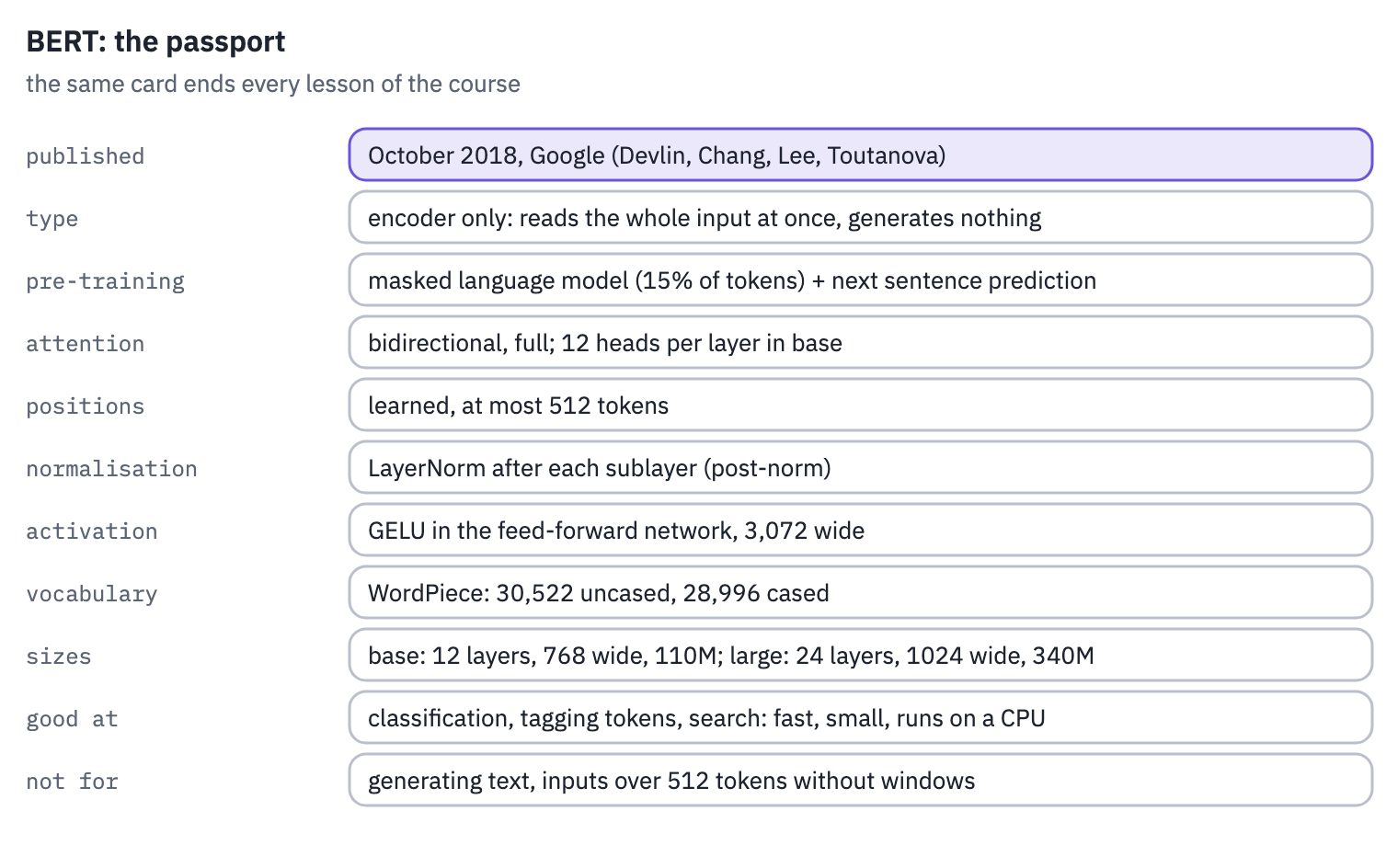
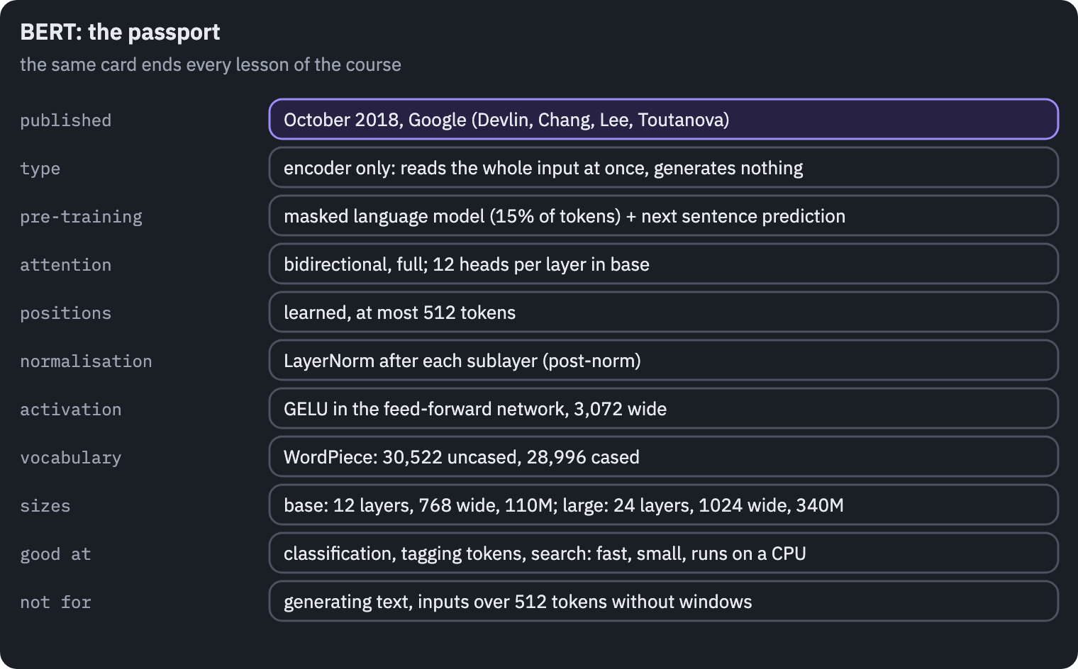
Every lesson of this course ends with the same card, the architecture’s passport, so that the models can be compared side by side:
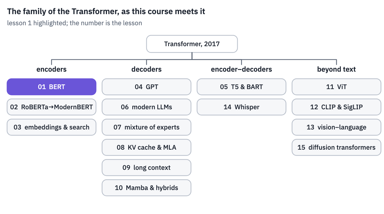
and with the family tree, which grows by one branch per lesson:
References
- Nayak, P. (2019). Understanding searches better than ever before. Google, 25 October 2019. ↩
- Devlin, J., Chang, M.-W., Lee, K., & Toutanova, K. (2018). BERT: pre-training of deep bidirectional transformers for language understanding. NAACL 2019. ↩
- Peters, M. E., Neumann, M., Iyyer, M., Gardner, M., Clark, C., Lee, K., & Zettlemoyer, L. (2018). Deep contextualized word representations. NAACL 2018. ↩
- Radford, A., Narasimhan, K., Salimans, T., & Sutskever, I. (2018). Improving language understanding by generative pre-training. OpenAI. ↩
- Taylor, W. L. (1953). “Cloze procedure”: a new tool for measuring readability. Journalism Quarterly, 30(4), 415–433. ↩
- Petroni, F., Rocktäschel, T., Lewis, P., Bakhtin, A., Wu, Y., Miller, A. H., & Riedel, S. (2019). Language models as knowledge bases? EMNLP 2019. ↩
- Kassner, N., & Schütze, H. (2020). Negated and misprimed probes for pretrained language models: birds can talk, but cannot fly. ACL 2020. ↩
- Kurita, K., Vyas, N., Pareek, A., Black, A. W., & Tsvetkov, Y. (2019). Measuring bias in contextualized word representations. 1st Workshop on Gender Bias in Natural Language Processing. ↩
- Clark, K., Khandelwal, U., Levy, O., & Manning, C. D. (2019). What does BERT look at? An analysis of BERT’s attention. BlackboxNLP 2019. ↩
- Gretel (2024). Synthetic PII finance multilingual. Hugging Face dataset, Apache 2.0. ↩