Contents
Transformers: from scratch to production · lesson 6 of 9 · all lessons · run on Kaggle · open in Colab · code on GitHub
Meta trained Llama 3 405B on up to sixteen thousand H100 GPUs; its model card counts 30.84 million GPU hours. Nobody tunes a run like that by trying things out. The paper’s learning rate, \(8 \times 10^{-5}\) with 8,000 steps of warm-up, and the size of the model itself were chosen on much smaller models and extrapolated [1]. OpenAI said the same of GPT-4: “for very large training runs like GPT-4, it is not feasible to do extensive model-specific tuning” [2].
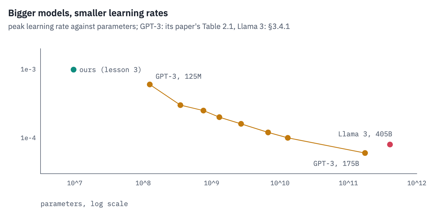
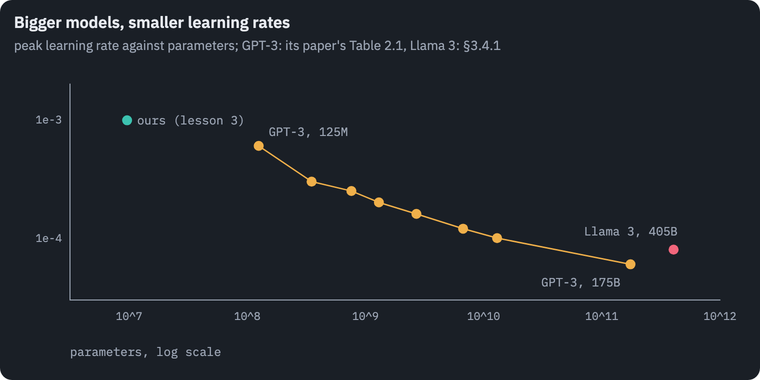
Each GPT-3 model got a learning rate of its own, larger the smaller the model, and ours sits roughly on the extension of that line. It got there by accident: its learning rate came from a formula in the 2017 paper, written for a model several times its size, and nobody has checked it since lesson 3.
That matters more than it sounds. In 2018 Melis et al. retuned the language models of the day with thousands of automatic trials and found that “LSTMs outperform the more recent models, contra the published claims”: a good part of the published progress had been tuning[3].
Lesson 5 compared architectures at one learning rate. This lesson asks what the settings themselves are worth, and spends an hour of a free GPU finding out.
What you’ll do
- Track every training run with Weights & Biases, with or without an account.
- Find the range of learning rates that work, for the 2017 design and for lesson 5’s, in a minute each.
- Write random search and successive halving from scratch and spend a fixed GPU budget on them.
- Train the winner to the end and check it against lesson 5’s model, with the bootstrap and with lesson 5’s seed runs.
- Run the same kind of search as a W&B Sweep, with Bayesian optimization and early stopping, and publish the tuned model.
What you need: a GPU. On Kaggle, Settings → Accelerator → GPU; on Colab, Runtime → Change runtime type → T4 GPU.
A free Weights & Biases account is optional: add your API key as the secret WANDB_API_KEY (Kaggle: Add-ons → Secrets; Colab: the key icon on the left) to see the runs online and run the sweep of section 8.
Without it everything else runs the same, and the runs are kept on disk. The notebook runs in about an hour and ten minutes.
Setup
One small helper package, tfs, draws the course’s plots and token chips and knows where the notebook runs (Kaggle, Colab or your own machine). Everything the lesson teaches is written out in the notebook itself.
import importlib.util
import subprocess
import sys

TFS = "git+https://github.com/xmarva/transformers-from-scratch@main"
if importlib.util.find_spec("tfs") is None:
    subprocess.check_call([sys.executable, "-m", "pip", "install", "-q", TFS])

from tfs import env
from tfs.viz import table, token_chips, use_course_style

env.quiet()  # no progress bars or environment warnings in the outputs
SEED = 42
env.seed_everything(SEED)
COLORS = use_course_style()
WORK_DIR = env.work_dir()
import json
import math
import os
import random
import time

import matplotlib.pyplot as plt
import numpy as np
import pandas as pd
import torch
from huggingface_hub import HfApi, hf_hub_download
from safetensors.torch import load_file, save_file
from tfs import decoding, training
from tfs.comet import Comet
from tfs.modern import Seq2Seq
from tokenizers import Tokenizer

for package in ["wandb", "sacrebleu"]:  # Kaggle has wandb, Colab may not
    if importlib.util.find_spec(package) is None:
        subprocess.check_call([sys.executable, "-m", "pip", "install", "-q", package])
import sacrebleu
import wandb

SMOKE = env.smoke()  # CI runs the lesson on a small slice; you tune in full
device = "cuda" if torch.cuda.is_available() else "cpu"
assert device == "cuda" or SMOKE, "This lesson trains two dozen models: switch to a GPU."
if device == "cuda":
    print("GPU:", torch.cuda.get_device_name(0))

WANDB_KEY = env.secret("WANDB_API_KEY")
if WANDB_KEY:
    os.environ["WANDB_API_KEY"] = WANDB_KEY
WANDB_MODE = "online" if WANDB_KEY and not SMOKE else "offline"
os.environ["WANDB_SILENT"] = "true"  # wandb's own messages stay out of the outputs
PROJECT = "transformers-from-scratch"  # one W&B project for the whole course
print("W&B:", WANDB_MODE)
GPU: Tesla T4
W&B: online
1. What we tune, and what we can spend
Five knobs: the peak learning rate and the warm-up of the schedule, dropout, label smoothing, and the size of a batch in tokens. Lesson 3 took all five from the 2017 paper.
The budget: Kaggle gives a free account about 30 hours of GPU a week, and Colab promises nothing at all. An epoch of our model takes about a minute on a T4 (lesson 5), so an hour buys some sixty epochs, three trainings of the length of lesson 3’s. Tuning on a budget is mostly deciding what not to train.
The data, the tokenizer and the batches, as in lesson 5. Since the batch size is one of the things we tune, the training pairs are cut into batches of three sizes, once:
tokenizer_path = hf_hub_download("xmarva/tfs-bpe-en-ru-16k", "tokenizer.json")
tokenizer = Tokenizer.from_file(tokenizer_path)
splits = {}
for name in ["train", "validation", "test"]:
    path = hf_hub_download("xmarva/tfs-tatoeba-en-ru", f"data/{name}.parquet",
                           repo_type="dataset")
    splits[name] = pd.read_parquet(path)
train, valid, test = splits["train"], splits["validation"], splits["test"]
if SMOKE:
    train = train.sample(3_000, random_state=SEED)
    valid = valid.head(300)
    test = test.sample(300, random_state=SEED)

VOCAB_SIZE = tokenizer.get_vocab_size()
PAD = tokenizer.token_to_id("<pad>")
BOS = tokenizer.token_to_id("<bos>")
EOS = tokenizer.token_to_id("<eos>")


def encode_all(sentences):
    return [encoding.ids for encoding in tokenizer.encode_batch(list(sentences))]


train_src, train_tgt = encode_all(train.en), encode_all(train.ru)
valid_src, valid_tgt = encode_all(valid.en), encode_all(valid.ru)
keep = []
for i in range(len(train_src)):
    if len(train_src[i]) <= 64 and len(train_tgt[i]) + 1 <= 64:
        keep.append(i)

special = {"pad_id": PAD, "bos_id": BOS, "eos_id": EOS}
BATCH_TOKENS = [3_000, 6_000, 12_000]  # lesson 3 used 6,000
batches = {}
for tokens in BATCH_TOKENS:
    batches[tokens] = training.make_batches(train_src, train_tgt, keep, tokens, **special)
valid_rows = range(len(valid_src))
valid_batches = training.make_batches(valid_src, valid_tgt, valid_rows, 6_000, **special)
for tokens in BATCH_TOKENS:
    print(f"batches of {tokens:,} tokens: {len(batches[tokens])} per epoch")
batches of 3,000 tokens: 1611 per epoch
batches of 6,000 tokens: 814 per epoch
batches of 12,000 tokens: 415 per epoch
The model is lesson 5’s, from tfs.modern: pre-norm with RMSNorm, SwiGLU and RoPE. For comparison, the 2017 design is one switch away.
LLAMA_STYLE = {"norm": "rms", "ffn": "swiglu", "pos": "rope"}
DESIGN_2017 = {"norm": "post", "ffn": "relu", "pos": "sinusoidal"}


def new_model(setup=LLAMA_STYLE, dropout=0.1, seed=SEED):
    torch.manual_seed(seed)
    return Seq2Seq(setup, VOCAB_SIZE, dropout=dropout, pad_id=PAD).to(device)
2. Tracking runs with Weights & Biases
Lessons 3 to 5 kept their results in print statements: a validation loss per epoch, scrolled past and gone.
With two dozen runs ahead that stops working. Weights & Biases (W&B) is an experiment tracker: every run records its configuration, everything you log, the load on the machine and the version of the code, and shows the runs side by side.
Four calls are all it takes: wandb.init starts a run with its configuration, run.log adds a row of numbers, run.summary keeps the final ones, run.finish closes the run. Without a key the same calls write to disk (mode="offline"), and wandb sync uploads them later. One epoch of lesson 5’s recipe, measured after each half:
run = wandb.init(project=PROJECT, mode=WANDB_MODE,
                 name="lesson 6: lesson 5's recipe, one epoch",
                 config={"peak_lr": 1e-3, "warmup": 1_000, "dropout": 0.1,
                         "label_smoothing": 0.1, "batch_tokens": 6_000})
config = run.config  # the hyperparameters, stored with the run

random.seed(SEED)
model = new_model(dropout=config.dropout)
optimizer = training.adam(model)


def schedule(step):
    return config.peak_lr * min(step / config.warmup, math.sqrt(config.warmup / step))


half_epoch = len(batches[config.batch_tokens]) // 2
steps = 0
for half in range(1, 3):  # two halves of an epoch, measured after each
    losses = training.train_steps(model, optimizer, batches[config.batch_tokens], schedule,
                                  half_epoch, pad_id=PAD, first_step=steps + 1,
                                  label_smoothing=config.label_smoothing, device=device)
    steps += len(losses)
    loss = training.validation_loss(model, valid_batches, pad_id=PAD, device=device)
    run.log({"epochs": half / 2, "train loss": np.mean(losses), "validation loss": loss})
A table of translations goes with the run too, so that the numbers come with something to read:
probe = test.sample(8, random_state=SEED)
written = decoding.greedy(model, tokenizer, list(probe.en))
translations = wandb.Table(columns=["English", "reference", "after one epoch"],
                           data=[list(row) for row in zip(probe.en, probe.ru, written)])
run.log({"translations": translations})
run.summary["validation loss"] = loss
print("validation loss after one epoch:", round(loss, 3))
print("stored in:", run.url if WANDB_MODE == "online" else run.dir)
run.finish()
validation loss after one epoch: 3.046
stored in: https://wandb.ai/ml-samurai/transformers-from-scratch/runs/mfy3yxjm
With a key, the run is a page in your W&B project: the curves, the configuration, the table of translations. The runs this notebook made when it was published are in a public project of the course, ml-samurai/transformers-from-scratch, to compare with yours.
3. The learning rate first
Of all the settings, the learning rate matters most, and it comes with the most quoted sentence of the field’s folklore: “This is often the single most important hyper-parameter and one should always make sure that it has been tuned”[4]. Before searching for it, find out where to search.
A learning-rate range test finds the range in one short run. Smith (2017) raised the learning rate linearly and watched the accuracy; the version most people use, from the fastai library, multiplies it by the same factor at every step, so that it sweeps several orders of magnitude, and watches the loss.
While the rate is too small, nothing happens; in the useful range the loss falls fast; beyond it, training breaks down.
def range_test(setup, start=1e-6, end=1.0, n_steps=600):
    random.seed(SEED)
    model = new_model(setup)
    optimizer = training.adam(model)
    factor = (end / start) ** (1 / n_steps)  # the same multiplication at every step

    def sweep_rate(step):
        return start * factor ** (step - 1)

    losses = training.train_steps(model, optimizer, batches[6_000], sweep_rate, n_steps,
                                  pad_id=PAD, device=device)
    rates = [sweep_rate(step) for step in range(1, len(losses) + 1)]
    return rates, losses


RANGE_STEPS = 600 if not SMOKE else 20
ranges = {}
for name, setup in [("2017 design", DESIGN_2017), ("lesson 5's design", LLAMA_STYLE)]:
    ranges[name] = range_test(setup, n_steps=RANGE_STEPS)
def until_diverged(rates, losses):
    """The test ends where the loss stops being a number, and so does the curve."""
    losses = np.asarray(losses, dtype=float)
    broken = np.flatnonzero(~np.isfinite(losses))
    end = broken[0] if len(broken) else len(losses)
    smooth = pd.Series(losses[:end]).rolling(15, min_periods=1).mean().to_numpy()
    return np.asarray(rates[:end]), smooth


fig, ax = plt.subplots(figsize=(6.4, 3.4))
for (name, (rates, losses)), color in zip(ranges.items(), [COLORS["muted"], COLORS["att"]]):
    rates, smooth = until_diverged(rates, losses)
    ax.plot(rates, smooth, color=color, label=name)
ax.set_xscale("log")
ax.set_ylim(top=12)
ax.set_xlabel("learning rate (rising every step)")
ax.set_ylabel("training loss, smoothed")
ax.set_title("A learning-rate range test")
ax.legend()
plt.show()

for name, (rates, losses) in ranges.items():
    rates, smooth = until_diverged(rates, losses)
    best_rate = rates[int(np.argmin(smooth))]
    print(f"{name}: lowest loss at a learning rate of {best_rate:.1e}")
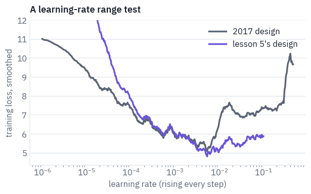
2017 design: lowest loss at a learning rate of 5.4e-03
lesson 5's design: lowest loss at a learning rate of 5.4e-03
Both models learn fastest around the same learning rate, a few times \(10^{-3}\), well above lesson 3’s peak. The difference is where they break. The 2017 design falls apart at a learning rate many times lower than lesson 5’s design does.
That is pre-norm’s gift, which lesson 5’s ablation couldn’t see: not a better model, a wider range of learning rates that work, which makes a model easier to tune and harder to break. At Llama’s scale, where a diverged run costs millions, that is the point.
4. Random search
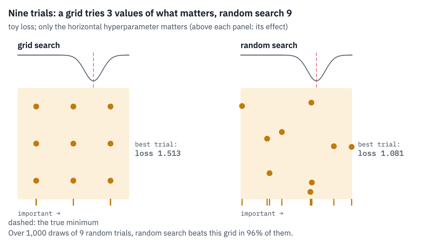
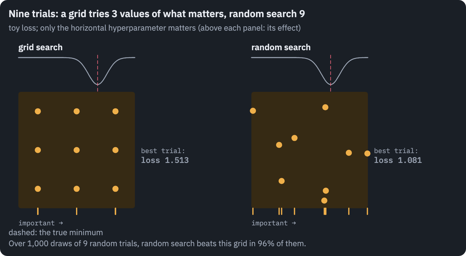
Five knobs, each with a range. The obvious search is a grid: three values of each, every combination, \(3^5 = 243\) runs, four days of our GPU. Random search draws every setting at random instead, and Bergstra and Bengio (2012) showed it is the better use of the same number of trials.
Usually only a few knobs matter, and a grid spends its trials repeating the same few values of exactly those:
The ranges. The learning rate and the warm-up are drawn on a logarithmic scale, since going from \(10^{-4}\) to \(2 \cdot 10^{-4}\) is as big a step as from \(10^{-3}\) to \(2 \cdot 10^{-3}\); dropout and label smoothing on a linear one; the batch from three sizes. Eighteen configurations, the first six of them:
search_rng = random.Random(SEED)


def log_uniform(low, high):
    return 10 ** search_rng.uniform(math.log10(low), math.log10(high))


def sample_config():
    return {
        "peak_lr": log_uniform(2e-4, 1e-2),
        "warmup": int(log_uniform(200, 4_000)),
        "dropout": search_rng.uniform(0.0, 0.3),
        "label_smoothing": search_rng.uniform(0.0, 0.2),
        "batch_tokens": search_rng.choice(BATCH_TOKENS),
    }


N_CONFIGS = 18 if not SMOKE else 3
configs = [sample_config() for _ in range(N_CONFIGS)]
table(pd.DataFrame(configs).head(6), digits=4)
| peak_lr | warmup | dropout | label_smoothing | batch_tokens |
|---|---|---|---|---|
| 0.0024 | 215 | 0.0825 | 0.0446 | 12,000 |
| 0.0003 | 1,839 | 0.1636 | 0.1181 | 3,000 |
| 0.0002 | 385 | 0.1516 | 0.0053 | 3,000 |
| 0.0033 | 1,634 | 0.1259 | 0.0898 | 6,000 |
| 0.0047 | 203 | 0.2417 | 0.1396 | 6,000 |
| 0.0006 | 381 | 0.2290 | 0.0204 | 6,000 |
5. Successive halving
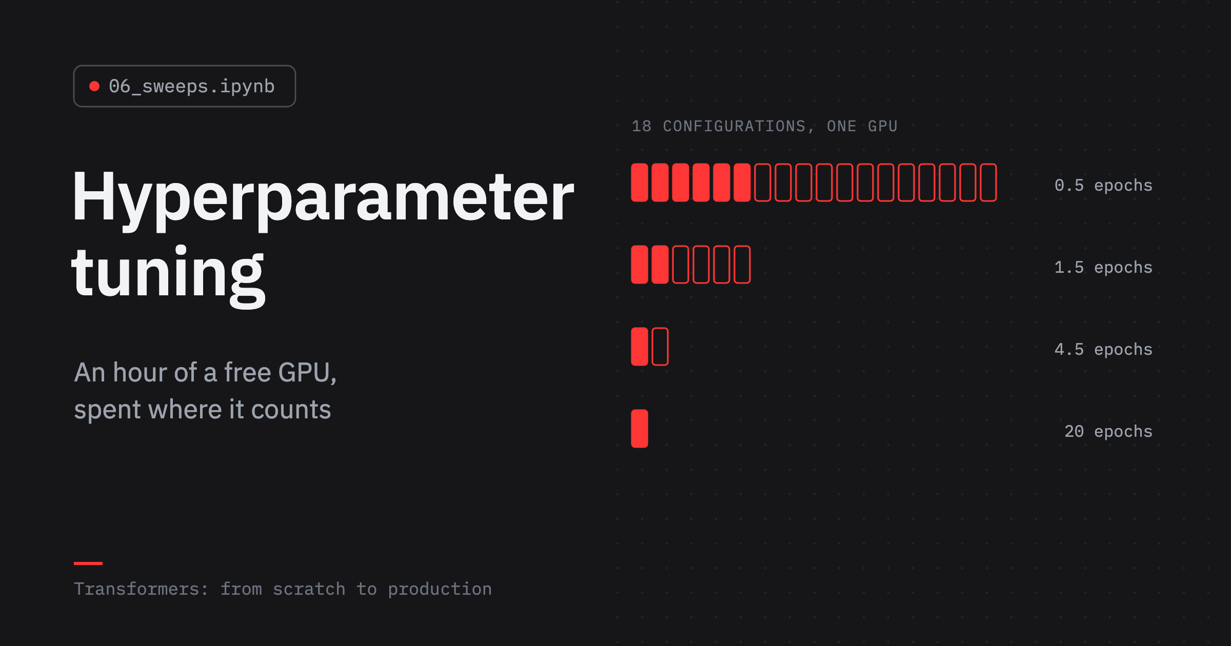
Eighteen configurations trained to the end would be eighteen trainings. But most configurations show early that they are no good: a learning rate that diverges does so in the first minutes. Successive halving [5] uses that: train every configuration a little, keep the best third, train those three times longer, keep the best third again. Hyperband[6] runs several such brackets, from many short trials to a few long ones, because nobody knows in advance how early the good ones show; we run one.
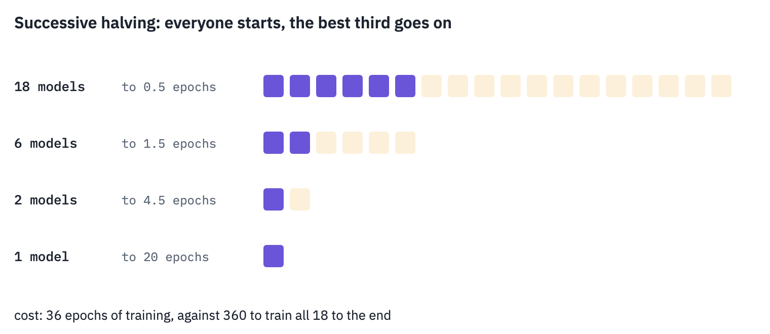
A trial is one configuration with its own model, optimizer and W&B run, able to train for a given number of half-epochs and to pick up where it stopped:
class Trial:
    def __init__(self, number, config, run=None):
        self.number, self.config = number, config
        self.model = new_model(dropout=config["dropout"], seed=SEED + number)
        self.optimizer = training.adam(self.model)
        self.steps, self.epochs, self.history = 0, 0.0, []
        if run is None:  # every trial is a W&B run of its own, all of them open at once
            run = wandb.init(project=PROJECT, mode=WANDB_MODE,
                             group="lesson 6: successive halving", name=f"trial {number}",
                             config=config, reinit="create_new")
        self.run = run

    def schedule(self, step):
        warmup, peak = self.config["warmup"], self.config["peak_lr"]
        return peak * min(step / warmup, math.sqrt(warmup / step))

    def train(self, half_epochs):
        own_batches = batches[self.config["batch_tokens"]]
        n_steps = max(1, int(len(own_batches) / 2 * half_epochs))
        smoothing = self.config["label_smoothing"]
        training.train_steps(self.model, self.optimizer, own_batches, self.schedule,
                             n_steps, pad_id=PAD, first_step=self.steps + 1,
                             label_smoothing=smoothing, device=device)
        self.steps += n_steps
        self.epochs += half_epochs / 2
        loss = training.validation_loss(self.model, valid_batches, pad_id=PAD,
                                        device=device)
        self.history.append({"epochs": self.epochs, "validation loss": loss})
        self.run.log({"epochs": self.epochs, "validation loss": loss})
        return loss
And the search: every rung trains the survivors up to its budget, ranks them by validation loss and keeps the best third. This is the long cell of the lesson.
RUNGS = [1, 3, 9]  # cumulative budget of each rung, in half-epochs
KEEP = 3  # keep the best 1 / KEEP

trials = [Trial(number, config) for number, config in enumerate(configs)]
survivors = list(trials)
done = 0
start = time.perf_counter()
for rung, budget in enumerate(RUNGS):
    for trial in survivors:
        trial.train(budget - done)
    done = budget
    survivors.sort(key=lambda trial: trial.history[-1]["validation loss"])
    minutes = (time.perf_counter() - start) / 60
    print("rung", rung, "|", len(survivors), "trials at", budget / 2, "epochs |",
          round(minutes), "min")
    if rung < len(RUNGS) - 1:
        survivors = survivors[: max(1, len(survivors) // KEEP)]
winner = survivors[0]
rung 0 | 18 trials at 0.5 epochs | 11 min
rung 1 | 6 trials at 1.5 epochs | 18 min
rung 2 | 2 trials at 4.5 epochs | 24 minfig, ax = plt.subplots(figsize=(6.4, 3.6))
for trial in trials:
epochs = [record["epochs"] for record in trial.history]
losses = [record["validation loss"] for record in trial.history]
is_winner = trial is winner
color = COLORS["att"] if is_winner else COLORS["line"]
width = 2 if is_winner else 1
ax.plot(epochs, losses, marker="o", markersize=3, color=color, linewidth=width)
ax.set_xlabel("epochs")
ax.set_ylabel("validation loss")
ax.set_ylim(top=min(6, ax.get_ylim()[1]))
ax.set_title("Eighteen starts, one finish")
plt.show()
rows = []
def furthest_first(trial): # the longest-trained first, then by their last loss
return (-trial.epochs, trial.history[-1]["validation loss"])
for trial in sorted(trials, key=furthest_first)[:6]:
rows.append({"trial": trial.number, "epochs": trial.epochs,
"validation loss": trial.history[-1]["validation loss"], **trial.config})
table(pd.DataFrame(rows), digits=4)
| trial | epochs | validation loss | peak_lr | warmup | dropout | label_smoothing | batch_tokens |
|---|---|---|---|---|---|---|---|
| 3 | 4.5000 | 1.2199 | 0.0033 | 1,634 | 0.1259 | 0.0898 | 6,000 |
| 0 | 4.5000 | 1.2245 | 0.0024 | 215 | 0.0825 | 0.0446 | 12,000 |
| 7 | 1.5000 | 1.9927 | 0.0012 | 290 | 0.2767 | 0.0158 | 6,000 |
| 4 | 1.5000 | 2.4696 | 0.0047 | 203 | 0.2417 | 0.1396 | 6,000 |
| 10 | 1.5000 | 2.5332 | 0.0059 | 624 | 0.1360 | 0.1668 | 3,000 |
| 2 | 1.5000 | 3.1484 | 0.0002 | 385 | 0.1516 | 0.0053 | 3,000 |
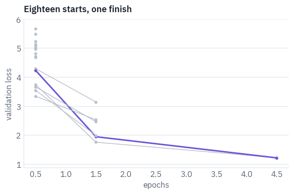
Watch the order change between rungs. After half an epoch the leaders are the fast starters: high learning rates, short warm-ups, small batches, which get more steps into the same half epoch. The configuration that wins at the end needn’t be among them.
Decisions made on short runs favour whatever pays off early; the problem has a name, short-horizon bias[7], and it is the price of stopping early. Keeping a third at every rung rather than a tenth is our insurance against it.
6. What mattered
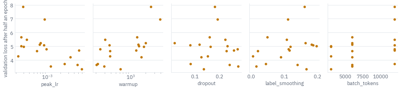
Every configuration ran at least half an epoch, so the first rung is a small random-search dataset: eighteen settings and their losses. Each knob against the loss:
first_rung = pd.DataFrame([{**trial.config, "loss": trial.history[0]["validation loss"]}
                           for trial in trials])
names = ["peak_lr", "warmup", "dropout", "label_smoothing", "batch_tokens"]
fig, axes = plt.subplots(1, len(names), figsize=(12, 2.8), sharey=True)
for ax, name in zip(axes, names):
    ax.scatter(first_rung[name], first_rung["loss"], color=COLORS["data"], s=18)
    if name in ["peak_lr", "warmup"]:
        ax.set_xscale("log")
    ax.set_xlabel(name)
axes[0].set_ylabel("validation loss after half an epoch")
plt.tight_layout()
plt.show()

# rank correlation: replace every value by its rank, then the usual correlation
correlations = first_rung[names].rank().corrwith(first_rung["loss"].rank())
table(pd.DataFrame({"hyperparameter": names,
                   "rank correlation with the loss": correlations.values}), digits=2)
| hyperparameter | rank correlation with the loss |
|---|---|
| peak_lr | -0.59 |
| warmup | 0.59 |
| dropout | -0.16 |
| label_smoothing | 0.28 |
| batch_tokens | 0.38 |
After half an epoch the learning rate and the warm-up dominate: higher peaks and shorter warm-ups mean a lower loss, the fast starters again.
Dropout barely matters yet. It fights overfitting, and half an epoch in there is nothing to overfit. These correlations describe the first minutes of training, not its end, which is the same bias as above, in numbers.
7. The winner, trained to the end
The winner of section 5 has trained for four and a half epochs. Successive halving’s last step is to let the survivor finish: one epoch at a time, to the twenty epochs of lessons 3 and 5, keeping the best weights.
FINAL_EPOCHS = 20 if not SMOKE else 1
CHECKPOINT = WORK_DIR / "tuned.safetensors"
best = winner.history[-1]["validation loss"]  # where the search left it
save_file(winner.model.state_dict(), CHECKPOINT)
while winner.epochs < FINAL_EPOCHS:
    loss = winner.train(2)  # one more epoch
    if loss < best:
        best = loss
        save_file(winner.model.state_dict(), CHECKPOINT)
for trial in trials:  # the search is over: its runs end here
    trial.run.finish()
tuned = winner.model
tuned.load_state_dict(load_file(CHECKPOINT, device=device))
tuned.eval()
print("best validation loss:", round(best, 4))
last_three = [round(record["validation loss"], 4) for record in winner.history[-3:]]
print("the last three epochs:", last_three)
table(pd.DataFrame([winner.config]), digits=4)
best validation loss: 0.9917
the last three epochs: [0.9917, 1.0037, 0.9997]| peak_lr | warmup | dropout | label_smoothing | batch_tokens |
|---|---|---|---|---|
| 0.0033 | 1,634 | 0.1259 | 0.0898 | 6,000 |
Lesson 5’s model, trained with the recipe of 2017, from the Hub, on the same validation set and the whole test set, with lesson 4’s metrics and the paired bootstrap:
LESSON5_REPO = "xmarva/tfs-transformer-en-ru-llama"
with open(hf_hub_download(LESSON5_REPO, "config.json")) as f:
    lesson5 = Seq2Seq(**json.load(f)).to(device).eval()
weights = hf_hub_download(LESSON5_REPO, "model.safetensors")
lesson5.load_state_dict(load_file(weights, device=device))

comet = Comet(device)
sentences = list(dict.fromkeys(test.en))
rows = []
for name, model in [("lesson 5", lesson5), ("tuned", tuned)]:
    translations = dict(zip(sentences, decoding.beam_search(model, tokenizer, sentences)))
    test[name] = test.en.map(translations)
    test[f"COMET {name}"] = comet.score(test.en, test[name], test.ru)
    loss = training.validation_loss(model, valid_batches, pad_id=PAD, device=device)
    rows.append({"model": name, "validation loss": loss,
                 "BLEU": sacrebleu.corpus_bleu(list(test[name]), [list(test.ru)]).score,
                 "chrF": sacrebleu.corpus_chrf(list(test[name]), [list(test.ru)]).score,
                 "COMET": test[f"COMET {name}"].mean()})
scores = pd.DataFrame(rows)
table(scores, digits=4)
| model | validation loss | BLEU | chrF | COMET |
|---|---|---|---|---|
| lesson 5 | 1.0283 | 41.5400 | 59.8959 | 0.8827 |
| tuned | 0.9917 | 42.1760 | 60.3722 | 0.8847 |
rng = np.random.default_rng(SEED)
a, b = test["COMET tuned"].to_numpy(), test["COMET lesson 5"].to_numpy()
differences = []
for _ in range(1_000):
    drawn = rng.integers(0, len(test), size=len(test))
    differences.append(a[drawn].mean() - b[drawn].mean())
low, high = np.percentile(differences, [2.5, 97.5])
print(f"COMET, tuned − lesson 5: {np.mean(differences):+.4f}")
print(f"95% of the draws between {low:+.4f} and {high:+.4f}")
COMET, tuned − lesson 5: +0.0021
95% of the draws between +0.0010 and +0.0031
About two thousandths of COMET, and the bootstrap keeps the whole interval above zero. Lesson 5 showed what the bootstrap can’t see: another training run of the same recipe lands somewhere else. Its seed runs include two more runs of lesson 5’s recipe at twenty epochs; here they are next to the model from the Hub and the tuned one:
SEED_RUNS = "xmarva/tfs-seed-runs-en-ru"
path = hf_hub_download(SEED_RUNS, "data/runs.parquet", repo_type="dataset")
seed_runs = pd.read_parquet(path)
recipe = seed_runs[(seed_runs.epochs == 20) & (seed_runs.setup == "+ RoPE")]
ours = scores.set_index("model")
rows = [{"model": "lesson 5, from the Hub",
         "validation loss": ours.loc["lesson 5", "validation loss"],
         "COMET": ours.loc["lesson 5", "COMET"]}]
for _, run in recipe.iterrows():
    rows.append({"model": f"lesson 5's recipe, seed {run.seed}",
                 "validation loss": run["validation loss"], "COMET": run.COMET})
rows.append({"model": "tuned", "validation loss": ours.loc["tuned", "validation loss"],
             "COMET": ours.loc["tuned", "COMET"]})
table(pd.DataFrame(rows), digits=4)
| model | validation loss | COMET |
|---|---|---|
| lesson 5, from the Hub | 1.0283 | 0.8827 |
| lesson 5's recipe, seed 43 | 1.0333 | 0.8818 |
| lesson 5's recipe, seed 44 | 1.0271 | 0.8827 |
| tuned | 0.9917 | 0.8847 |
Three runs of lesson 5’s recipe sit within about a thousandth of COMET of each other, and the tuned model is above all of them by more than they differ among themselves: the two thousandths come from the hyperparameters, not from the seed.
That is about half of what lesson 5’s four changes to the architecture bought over the 2017 design trained the same way. The validation loss moved much further than COMET did: a lower loss doesn’t turn one for one into better translations.
A search doesn’t replace a better model. It replaces a habit: lesson 5 trained a new architecture with the numbers of 2017, and they turned out to be close to right, not right.
One number escaped the search: twenty epochs, lesson 3’s budget, inherited and never searched over. The last three epochs printed above show the loss had stopped falling, so this time twenty was enough.
Where the two thousandths land, by the length of the English sentence:
encoded = tokenizer.encode_batch(list(test.en))
test["English tokens"] = [len(encoding.ids) for encoding in encoded]
edges = [0, 5, 8, 11, 15, 20, 30, 1000]
test["length"] = pd.cut(test["English tokens"], edges)
test["gain"] = test["COMET tuned"] - test["COMET lesson 5"]
test["same translation"] = test["tuned"] == test["lesson 5"]
by_length = test.groupby("length", observed=True).agg(
    sentences=("gain", "size"), same=("same translation", "mean"), gain=("gain", "mean"))

rows = []
for interval, row in by_length.iterrows():
    if interval.right == edges[-1]:
        tokens = f"over {interval.left}"
    else:
        tokens = f"{interval.left + 1}–{interval.right}"
    rows.append({"tokens": tokens, "sentences": int(row.sentences),
                 "same translation": f"{row.same:.0%}", "COMET gain": row.gain})
table(pd.DataFrame(rows), digits=4)
| tokens | sentences | same translation | COMET gain |
|---|---|---|---|
| 1–5 | 3,520 | 54% | 0.0023 |
| 6–8 | 15,656 | 47% | 0.0024 |
| 9–11 | 10,614 | 34% | 0.0010 |
| 12–15 | 4,383 | 21% | 0.0020 |
| 16–20 | 1,196 | 6% | 0.0007 |
| 21–30 | 576 | 1% | 0.0081 |
| over 30 | 440 | 0% | 0.0111 |
Half the shortest sentences come out word for word as lesson 5 wrote them, and up to twenty tokens the gain is a couple of thousandths or less.
Past twenty tokens the two models almost never agree, and the gain is several times larger, as it was for lesson 5’s architecture. Long sentences are rare in Tatoeba, so the average hides most of it.
8. The same search as a W&B Sweep
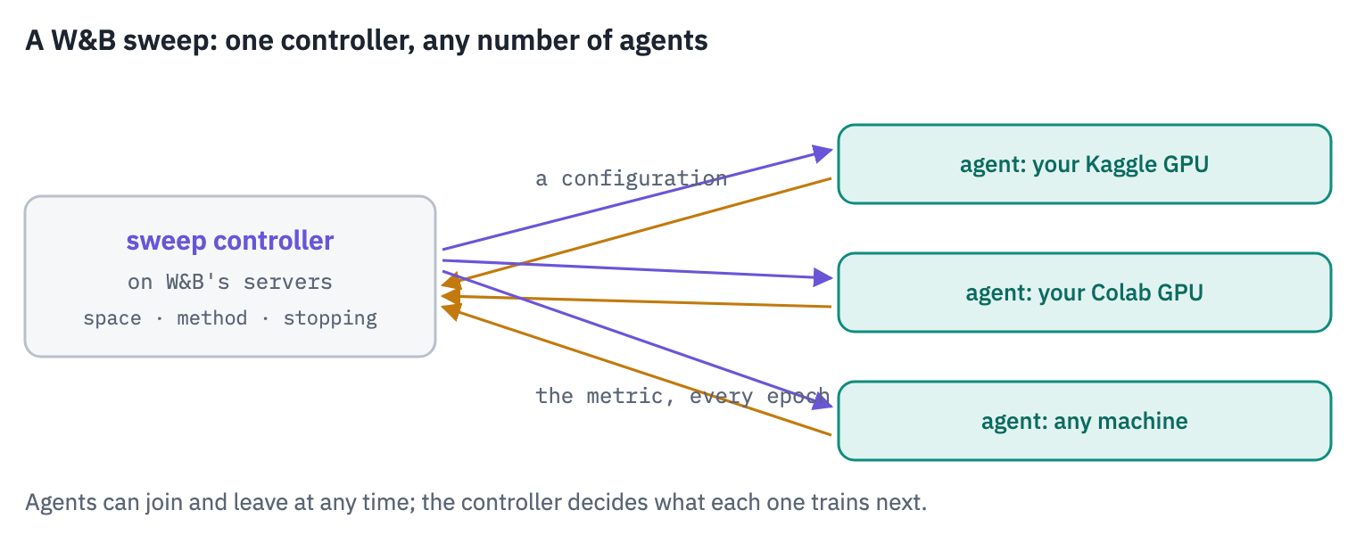
Our search ran in one notebook, one trial after another. W&B Sweeps moves the controller to a server: it holds the search space and the method, hands configurations out to agents, and stops runs that fall behind.
Any number of agents on any machines can work on one sweep, and that is how the same search goes from a free T4 to a cluster.
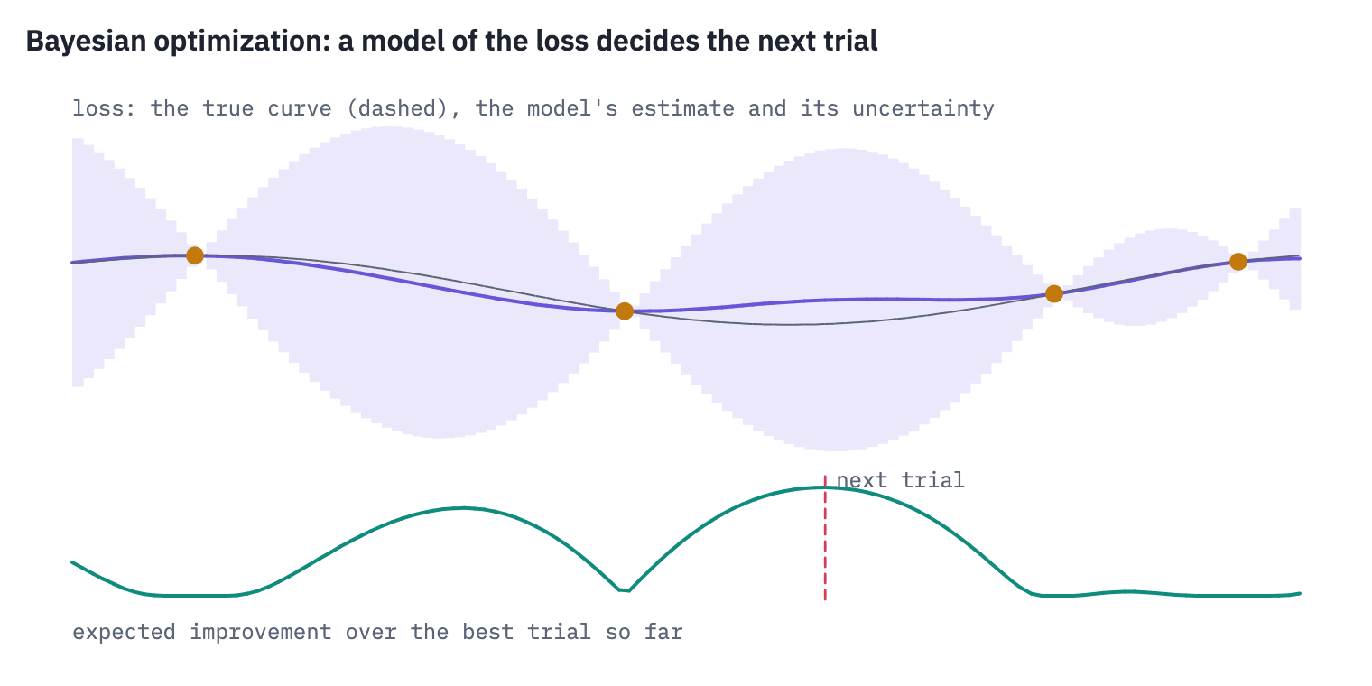
It can also search less blindly than at random. With method: bayes the controller fits a model of the loss as a function of the settings, a Gaussian process[8], and picks the next configuration where it expects the most improvement: where the predicted loss is low, or where the model is still unsure.
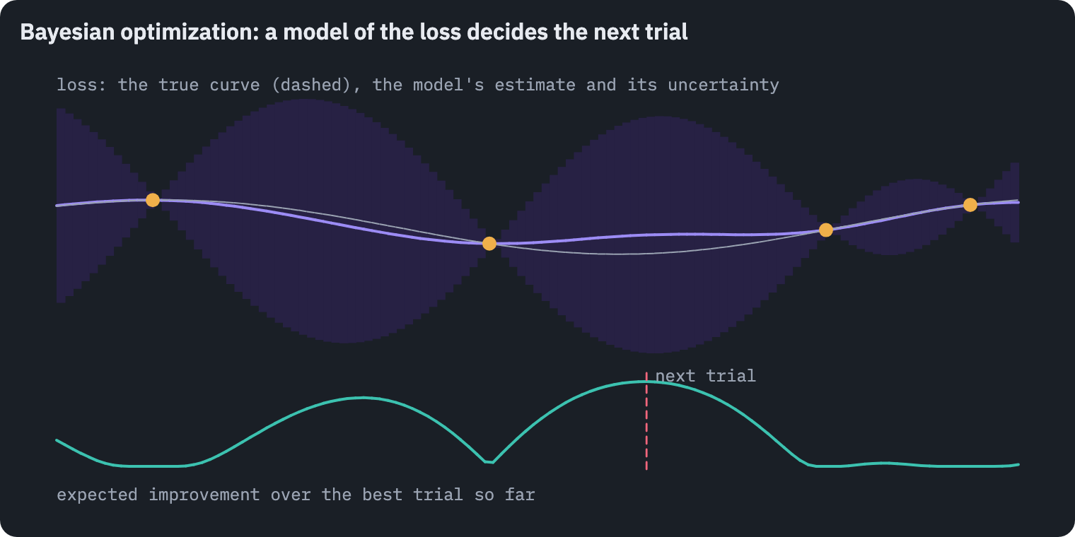
The search space in W&B’s terms is a dictionary, the same space as section 4:
SWEEP = {
    "method": "bayes",
    "metric": {"name": "validation loss", "goal": "minimize"},
    "parameters": {
        "peak_lr": {"distribution": "log_uniform_values", "min": 2e-4, "max": 1e-2},
        "warmup": {"distribution": "q_log_uniform_values", "min": 200, "max": 4_000,
                   "q": 1},
        "dropout": {"distribution": "uniform", "min": 0.0, "max": 0.3},
        "label_smoothing": {"distribution": "uniform", "min": 0.0, "max": 0.2},
        "batch_tokens": {"values": BATCH_TOKENS},
    },
    "early_terminate": {"type": "hyperband", "min_iter": 1, "eta": 3},
}
Each run of the sweep is a function the agent calls: it reads its configuration from W&B, trains for up to three half-epochs, and logs the validation loss after each, which is what the early stopping watches.
def sweep_run():
    with wandb.init() as run:  # the agent filled run.config with the controller's choice
        trial = Trial(0, dict(run.config), run=run)
        try:
            for _ in range(3):
                trial.train(1)
        except Exception as error:
            if type(error) is not Exception:  # a real error, not the controller's stop
                raise
            # early stopping: the agent stops a run by raising a bare Exception inside it
            print(f"{run.name}: stopped by the controller after {trial.epochs} epochs")


SWEEP_RUNS = 6
if WANDB_MODE == "online":
    sweep_id = wandb.sweep(SWEEP, project=PROJECT)
    wandb.agent(sweep_id, function=sweep_run, count=SWEEP_RUNS)
    swept = wandb.Api().sweep(f"{wandb.Api().default_entity}/{PROJECT}/{sweep_id}")
    rows = []
    for swept_run in swept.runs:
        rows.append({"run": swept_run.name, "state": swept_run.state,
                     "validation loss": swept_run.summary.get("validation loss"),
                     **{k: swept_run.config.get(k) for k in SWEEP["parameters"]}})
    print("the sweep:", swept.url)
    display(table(pd.DataFrame(rows).sort_values("validation loss"), digits=4))
else:
    print("no W&B key: the sweep needs W&B's servers, so this cell does nothing offline")
Create sweep with ID: hlu8vocf
Sweep URL: https://wandb.ai/ml-samurai/transformers-from-scratch/sweeps/hlu8vocf
volcanic-sweep-3: stopped by the controller after 1.0 epochs
proud-sweep-5: stopped by the controller after 1.0 epochs
the sweep: https://wandb.ai/ml-samurai/transformers-from-scratch/sweeps/hlu8vocf| run | state | validation loss | peak_lr | warmup | dropout | label_smoothing | batch_tokens |
|---|---|---|---|---|---|---|---|
| treasured-sweep-2 | finished | 1.5720 | 0.0035 | 264 | 0.0686 | 0.0256 | 6,000 |
| wobbly-sweep-4 | finished | 1.6742 | 0.0009 | 1,160 | 0.0189 | 0.0242 | 3,000 |
| youthful-sweep-6 | finished | 1.8412 | 0.0047 | 545 | 0.0019 | 0.0042 | 3,000 |
| zany-sweep-1 | finished | 2.6912 | 0.0007 | 3,783 | 0.1003 | 0.0896 | 3,000 |
| volcanic-sweep-3 | finished | 3.6500 | 0.0079 | 3,014 | 0.2736 | 0.1855 | 12,000 |
| proud-sweep-5 | finished | 3.7993 | 0.0003 | 237 | 0.0170 | 0.0144 | 6,000 |
Six runs give a Gaussian process little to model; Bayesian optimization pays off over dozens of trials, not a handful. Two details from W&B’s own source are worth knowing. The model is a Gaussian process with a Matérn kernel, choosing by expected improvement.
And the “hyperband” of the configuration is a simpler rule than the paper’s: when a run reports its metric for the \(n\)-th time, it is stopped if it is worse than the best third of the runs that got that far.
The lines above the table are that rule at work: the controller stopped the runs it judged hopeless after a report or two, and their GPU time went to the next configuration.
One thing here is not reproducible. W&B’s controller has no seed, so the sweep proposes other configurations every time the notebook runs, and its table changes with them; everything else in the lesson comes out the same.
What this section shows is the machinery: a search space in one dictionary, and as many GPUs as you can find.
9. Save and publish
MODEL_DIR = WORK_DIR / "model"
MODEL_DIR.mkdir(exist_ok=True)
save_file(tuned.state_dict(), MODEL_DIR / "model.safetensors")
TUNED_CONFIG = {"setup": LLAMA_STYLE, "vocab_size": VOCAB_SIZE, "d_model": 256,
                "n_heads": 4, "d_ff": 1024, "n_layers": 3,
                "dropout": winner.config["dropout"], "pad_id": PAD}
(MODEL_DIR / "config.json").write_text(json.dumps(TUNED_CONFIG, indent=2))
(MODEL_DIR / "training.json").write_text(json.dumps(winner.config, indent=2))
print("saved:", sorted(path.name for path in MODEL_DIR.iterdir()))
saved: ['config.json', 'model.safetensors', 'training.json']MODEL_CARD = f"""---
license: cc-by-2.0
language: [en, ru]
tags: [translation, transformer]
datasets: [xmarva/tfs-tatoeba-en-ru]
---
# A small English→Russian Transformer, tuned
Built in lesson 6 of the course "Transformers: from scratch to production":
https://github.com/xmarva/transformers-from-scratch
- lesson 5's model (pre-norm, RMSNorm, SwiGLU, RoPE), hyperparameters from a search
- the training hyperparameters: training.json
- best validation cross-entropy: {best:.3f}
"""
HUB_USER = os.environ.get("TFS_HUB_USER")
hf_token = env.secret("HF_TOKEN")
if HUB_USER and hf_token and not SMOKE:
api = HfApi(token=hf_token)
model_repo = f"{HUB_USER}/tfs-transformer-en-ru-tuned"
api.create_repo(model_repo, exist_ok=True)
api.upload_folder(folder_path=str(MODEL_DIR), repo_id=model_repo)
api.upload_file(path_or_fileobj=MODEL_CARD.encode(), path_in_repo="README.md",
repo_id=model_repo)
print("published", model_repo)
else:
print("not publishing; later lessons download the course's copy:")
print("xmarva/tfs-transformer-en-ru-tuned")
not publishing; later lessons download the course's copy:
xmarva/tfs-transformer-en-ru-tuned
References
- Llama Team, AI @ Meta (2024). The Llama 3 Herd of Models. Scaling laws for choosing the model size; the 405B learning rate. ↩
- OpenAI (2023). GPT-4 Technical Report. Predictable scaling. ↩
- Melis, G., Dyer, C., Blunsom, P. (2018). On the State of the Art of Evaluation in Neural Language Models. ICLR. ↩
- Bengio, Y. (2012). Practical Recommendations for Gradient-Based Training of Deep Architectures. ↩
- Jamieson, K., Talwalkar, A. (2016). Non-stochastic Best Arm Identification and Hyperparameter Optimization. AISTATS. Successive halving. ↩
- Li, L. et al. (2018). Hyperband: A Novel Bandit-Based Approach to Hyperparameter Optimization. JMLR. ↩
- Wu, Y., Ren, M., Liao, R., Grosse, R. (2018). Understanding Short-Horizon Bias in Stochastic Meta-Optimization. ICLR. ↩
- Snoek, J., Larochelle, H., Adams, R. P. (2012). Practical Bayesian Optimization of Machine Learning Algorithms. NeurIPS. ↩
- Brown, T. et al. (2020). Language Models are Few-Shot Learners. NeurIPS. Table 2.1: GPT-3’s learning rates.
- Smith, L. N. (2017). Cyclical Learning Rates for Training Neural Networks. WACV. The learning-rate range test.
- Bergstra, J., Bengio, Y. (2012). Random Search for Hyper-Parameter Optimization. JMLR.
- Yang, G. et al. (2022). Tensor Programs V: Tuning Large Neural Networks via Zero-Shot Hyperparameter Transfer. Tuning a small proxy instead of the large model.
- W&B Sweeps documentation and the sweeps source.