Contents
Transformers: from scratch to production · lesson 5 of 9 · all lessons · run on Kaggle · open in Colab · code on GitHub
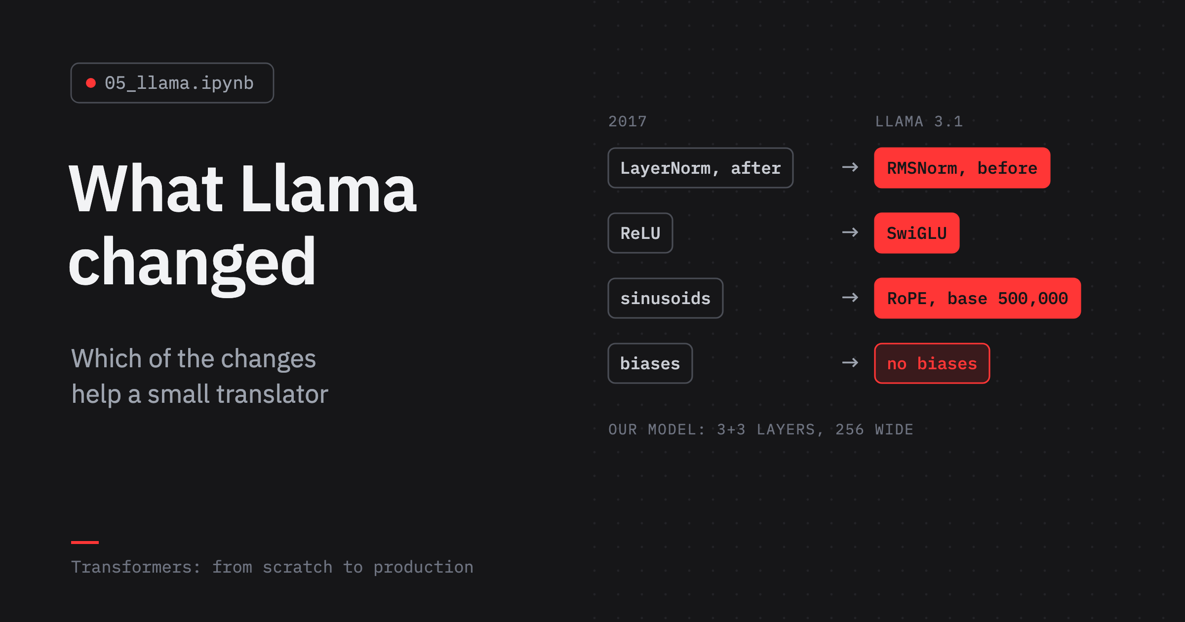
Llama 3.1, Meta’s open model family, goes up to 405 billion parameters. Its blueprint is the Transformer of 2017, the one you built in lesson 2, with a handful of details changed.
You don’t need to download sixteen gigabytes of weights to see which. The config file and the headers of the weight files say it all:
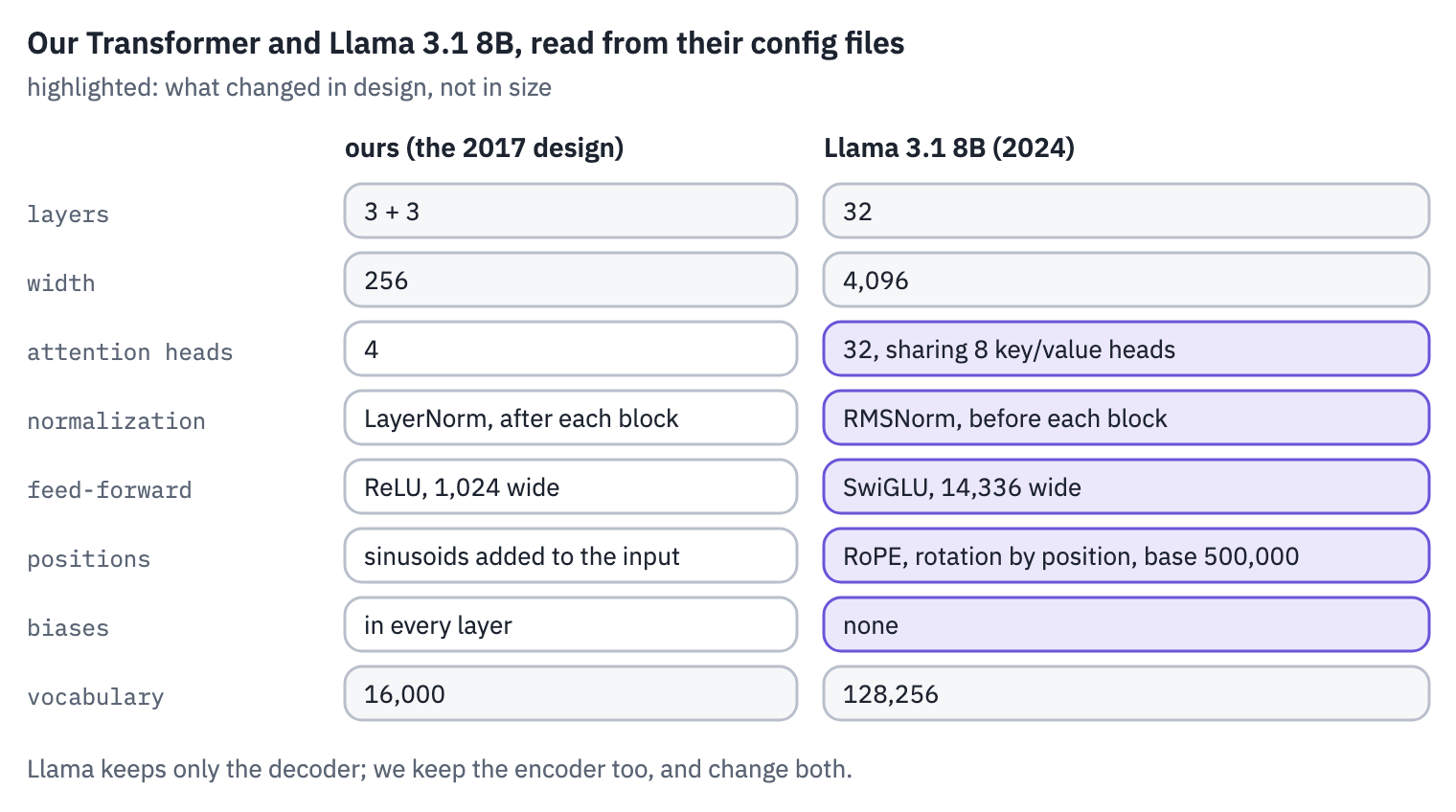
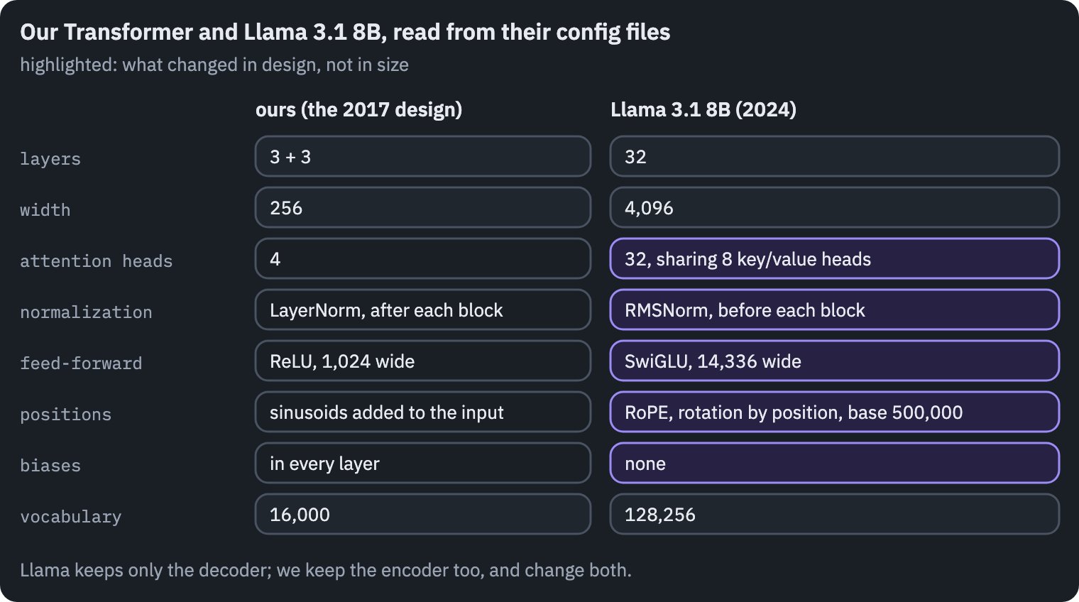
The size differs by a factor of a thousand, and nobody is surprised by that. Meta’s paper is frank about the rest: Llama 3 “uses a standard, dense Transformer architecture”, and its gains are “primarily driven by improvements in data quality and diversity as well as by increased training scale” [1]. The five highlighted rows are the more interesting part. Each is a change that survived years of people trying to improve the Transformer, and most such attempts didn’t survive: when a team at Google reimplemented dozens of published modifications in one codebase, most of them made no real difference[2].
So in this lesson we don’t take Llama’s choices on faith. We make them in our own translator, one at a time, train every version with the same budget, and judge them with the metrics and the bootstrap of lesson 4.
A change that helps a 7-billion-parameter chatbot doesn’t have to help a ten-million-parameter translator, and the only way to know is to measure.
What you’ll do
- Read Llama 3.1’s configuration and weight shapes without downloading its weights.
- Make training faster with fused attention, the first thing every modern implementation changes.
- Write pre-norm, RMSNorm, SwiGLU and rotary position embeddings, each checked against a reference.
- Train an ablation ladder: five models, one change apart, and see how much of what it shows a new seed undoes.
- Add a KV cache, train the final model with lesson 3’s full recipe, compare it with lesson 3’s, and publish it.
What you need: a GPU. On Kaggle, Settings → Accelerator → GPU; on Colab, Runtime → Change runtime type → T4 GPU.
The notebook downloads the data and tokenizer of lesson 1, the model of lesson 3, the COMET checkpoint of lesson 4 and the course’s seed runs, and trains ten models, most of them briefly; on a T4 it runs in about an hour and a quarter.
Setup
One small helper package, tfs, draws the course’s plots and token chips and knows where the notebook runs (Kaggle, Colab or your own machine). Everything the lesson teaches is written out in the notebook itself.
import importlib.util
import subprocess
import sys

TFS = "git+https://github.com/xmarva/transformers-from-scratch@main"
if importlib.util.find_spec("tfs") is None:
    subprocess.check_call([sys.executable, "-m", "pip", "install", "-q", TFS])

from tfs import env
from tfs.viz import table, token_chips, use_course_style

env.quiet()  # no progress bars or environment warnings in the outputs
SEED = 42
env.seed_everything(SEED)
COLORS = use_course_style()
WORK_DIR = env.work_dir()
import json
import math
import os
import random
import time

import matplotlib.pyplot as plt
import numpy as np
import pandas as pd
import torch
import torch.nn as nn
import torch.nn.functional as F
from huggingface_hub import HfApi, get_safetensors_metadata, hf_hub_download
from safetensors.torch import load_file, save_file
from tfs import decoding, training
from tfs.comet import Comet
from tfs.model import Transformer, positional_encoding
from tokenizers import Tokenizer

# sacreBLEU, the reference implementation of BLEU and chrF
if importlib.util.find_spec("sacrebleu") is None:
    pip = [sys.executable, "-m", "pip", "install", "-q"]
    subprocess.check_call(pip + ["sacrebleu==2.6.0"])
import sacrebleu

SMOKE = env.smoke()  # CI runs the lesson on a small slice; you train in full
device = "cuda" if torch.cuda.is_available() else "cpu"
assert device == "cuda" or SMOKE, "This lesson trains ten models: switch to a GPU."
if device == "cuda":
    print("GPU:", torch.cuda.get_device_name(0))
GPU: Tesla T41. Inside Llama 3.1
Meta’s own repository on the Hugging Face Hub asks you to accept a license before downloading. The files below come from an exact copy that doesn’t, and we read only the configuration, a few kilobytes:
LLAMA = "unsloth/Meta-Llama-3.1-8B-Instruct"  # Meta's Llama 3.1 8B, no license gate
with open(hf_hub_download(LLAMA, "config.json")) as f:
    llama = json.load(f)

FIELDS = ["num_hidden_layers", "hidden_size", "num_attention_heads", "num_key_value_heads",
          "intermediate_size", "hidden_act", "rms_norm_eps", "rope_theta", "vocab_size"]
table(pd.DataFrame({"setting": FIELDS, "value": [str(llama[name]) for name in FIELDS]}))
| setting | value |
|---|---|
| num_hidden_layers | 32 |
| hidden_size | 4096 |
| num_attention_heads | 32 |
| num_key_value_heads | 8 |
| intermediate_size | 14336 |
| hidden_act | silu |
| rms_norm_eps | 1e-05 |
| rope_theta | 500000.0 |
| vocab_size | 128256 |
The weights are stored in safetensors files, as ours are since lesson 3. Each file starts with a header that lists every tensor’s name, shape and type, and the Hub can serve just that header.
So the shape of every weight matrix is a few requests away. Here is the first of Llama’s 32 layers:
metadata = get_safetensors_metadata(LLAMA)
rows, total, biases = [], 0, []
for file_metadata in metadata.files_metadata.values():
    for name, tensor in file_metadata.tensors.items():
        total += math.prod(tensor.shape)
        if name.endswith("bias"):
            biases.append(name)
        if ".layers.0." in name:
            short = name.removeprefix("model.layers.0.")
            rows.append({"tensor": short, "shape": str(tensor.shape)})
print(f"parameters, counted from the headers: {total / 1e9:.2f} billion")
print("bias tensors:", len(biases))
table(pd.DataFrame(rows))
parameters, counted from the headers: 8.03 billion
bias tensors: 0| tensor | shape |
|---|---|
| input_layernorm.weight | [4096] |
| mlp.down_proj.weight | [4096, 14336] |
| mlp.gate_proj.weight | [14336, 4096] |
| mlp.up_proj.weight | [14336, 4096] |
| post_attention_layernorm.weight | [4096] |
| self_attn.k_proj.weight | [1024, 4096] |
| self_attn.o_proj.weight | [4096, 4096] |
| self_attn.q_proj.weight | [4096, 4096] |
| self_attn.v_proj.weight | [1024, 4096] |
Read the shapes like a spec sheet. The query projection is 4,096 × 4,096: 32 heads of 128 numbers.
The key and value projections are only 1,024 wide, 8 heads of 128: every four query heads share one key head and one value head. That’s grouped-query attention[3], and it makes what a model must remember per token while it writes (section 11) four times smaller.
The feed-forward layer has three matrices, gate, up and down: that’s SwiGLU (section 7). Each layer has two norms, each a single vector, a scale without a shift: RMSNorm (section 6).
They sit before the attention and before the feed-forward layer, which the names give away once you know that post_attention means “after attention, before the feed-forward layer”: pre-norm (section 5). Not a single bias in eight billion parameters. And no table of positions anywhere: RoPE computes them (section 8).
2. The plan
Of those five changes we make four. Grouped-query attention saves memory when a model has many heads and long contexts; with our four heads and sentences of a dozen tokens there is nothing to save.
And Llama keeps only a decoder, because it continues text. A translator reads a whole source sentence first, so ours keeps its encoder, and every change goes into both stacks.
The method is an ablation ladder: start from the 2017 design and make one change at a time, training every model for the same number of steps on the same data, from the same seed.
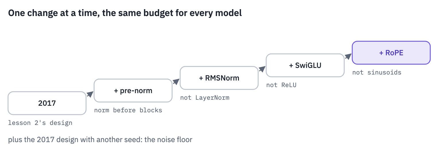
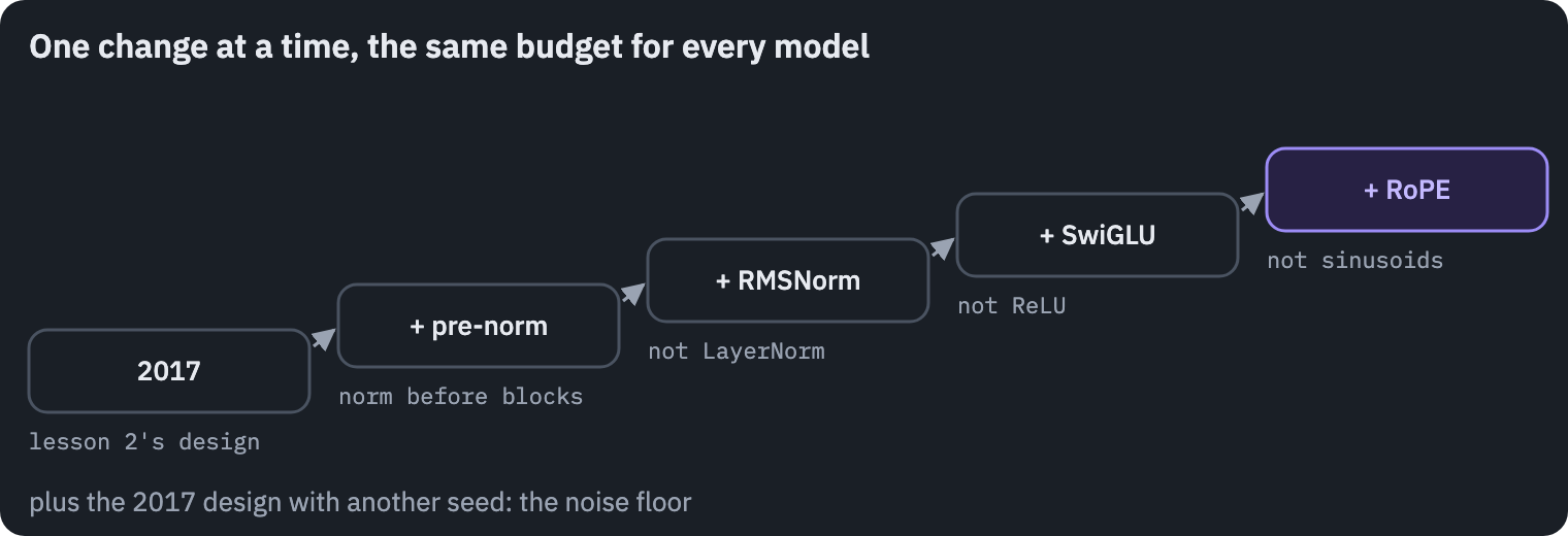
Each rung differs from the one before it by a single change, so a difference between neighbours belongs to that change. Almost: changes can interact, and the order of the rungs is a choice.
RMSNorm comes after pre-norm because Llama uses it in the pre-norm position. Testing every combination would take sixteen models; a free GPU affords six runs.
The sixth run is the most important one, and papers skip it surprisingly often: the 2017 design again, with another seed. The two 2017 runs differ by nothing but chance, so their difference is the yardstick for all the others.
3. Data, and the training loop of lesson 3
The data and tokenizer of lesson 1, from the Hub:
tokenizer_path = hf_hub_download("xmarva/tfs-bpe-en-ru-16k", "tokenizer.json")
tokenizer = Tokenizer.from_file(tokenizer_path)
splits = {}
for name in ["train", "validation", "test"]:
    path = hf_hub_download("xmarva/tfs-tatoeba-en-ru", f"data/{name}.parquet",
                           repo_type="dataset")
    splits[name] = pd.read_parquet(path)
train, valid, test = splits["train"], splits["validation"], splits["test"]
if SMOKE:
    train = train.sample(3_000, random_state=SEED)
    valid = valid.head(300)
    test = test.sample(300, random_state=SEED)

VOCAB_SIZE = tokenizer.get_vocab_size()
PAD = tokenizer.token_to_id("<pad>")
BOS = tokenizer.token_to_id("<bos>")
EOS = tokenizer.token_to_id("<eos>")
print("train:", len(train), "validation:", len(valid), "test:", len(test))
train: 508093 validation: 10370 test: 36385Lesson 3’s training loop is in the course package now, as tfs.training, unchanged: batches of about 6,000 tokens with sentences of similar length side by side, cross-entropy with label smoothing, Adam, gradient clipping and mixed precision.
def encode_all(sentences):
    return [encoding.ids for encoding in tokenizer.encode_batch(list(sentences))]


train_src, train_tgt = encode_all(train.en), encode_all(train.ru)
valid_src, valid_tgt = encode_all(valid.en), encode_all(valid.ru)

MAX_LEN = 64  # lesson 3 left out the few longer pairs
keep = []
for i in range(len(train_src)):
    if len(train_src[i]) <= MAX_LEN and len(train_tgt[i]) + 1 <= MAX_LEN:
        keep.append(i)

special = {"pad_id": PAD, "bos_id": BOS, "eos_id": EOS}
train_batches = training.make_batches(train_src, train_tgt, keep, 6_000, **special)
valid_rows = range(len(valid_src))
valid_batches = training.make_batches(valid_src, valid_tgt, valid_rows, 6_000, **special)
print("training batches:", len(train_batches), "validation batches:", len(valid_batches))
training batches: 814 validation batches: 224. Fused attention
Seven models are about to be trained, so start with the change that makes every one of them faster without changing a single result.
Lesson 2’s attention takes three steps, each one a separate pass over the GPU’s memory: compute the scores \(QK^\top\), a matrix of \(T \times T\) numbers per head, write it out; read it back for the softmax and write the weights; read them again to multiply by \(V\).
FlashAttention[4] computes exactly the same thing in tiles small enough to stay in the GPU’s fast on-chip memory, so the \(T \times T\) matrix never travels to the slow memory at all. The result is not an approximation; the arithmetic is merely reordered.
PyTorch ships such kernels behind one function, F.scaled_dot_product_attention, and picks the fastest one the GPU supports. On a T4 that isn’t FlashAttention itself, which needs a newer GPU, but a memory-efficient kernel that also works through the matrix piece by piece.
Lesson 2’s attention, with one change: the mask is now boolean, True where a position may be seen, which is what the fused function takes as well. Then the check that both compute the same:
def attention(q, k, v, mask=None):
    scores = q @ k.transpose(-2, -1) / math.sqrt(q.shape[-1])
    if mask is not None:
        scores = scores.masked_fill(~mask, float("-inf"))  # hidden positions get no weight
    return scores.softmax(dim=-1) @ v


q, k, v = (torch.randn(8, 4, 40, 64, device=device) for _ in range(3))
causal = torch.ones(40, 40, dtype=torch.bool, device=device).tril()[None, None]
ours = attention(q, k, v, causal)
fused = F.scaled_dot_product_attention(q, k, v, attn_mask=causal)
assert torch.allclose(ours, fused, atol=1e-5)
print("largest difference:", (ours - fused).abs().max().item())
largest difference: 5.960464477539062e-07Equal to rounding. How much faster it trains, section 9 measures on the whole model.
5. Pre-norm
Look at the residual stream: the vector \(x_l\) that flows through the stack of layers, each layer adding something to it. The 2017 design normalizes the stream after every addition; pre-norm normalizes only the copy that goes into the sublayer, and adds the result to the stream untouched:
\[\text{post-norm:}\quad x_{l+1} = \mathrm{Norm}\big(x_l + F_l(x_l)\big), \qquad \text{pre-norm:}\quad x_{l+1} = x_l + F_l\big(\mathrm{Norm}(x_l)\big).\]\(F_l\) is the sublayer, attention or feed-forward. Unroll the pre-norm version and the stream at the top is the input plus everything the layers added:
\[x_L = x_0 + \sum_{l=0}^{L-1} F_l\big(\mathrm{Norm}(x_l)\big).\]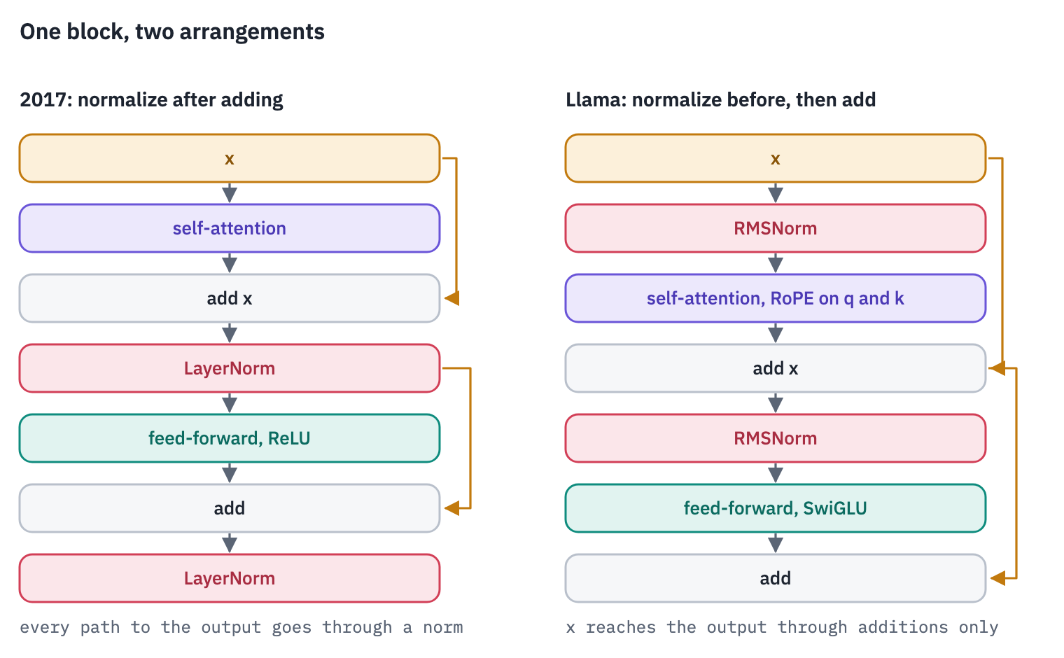
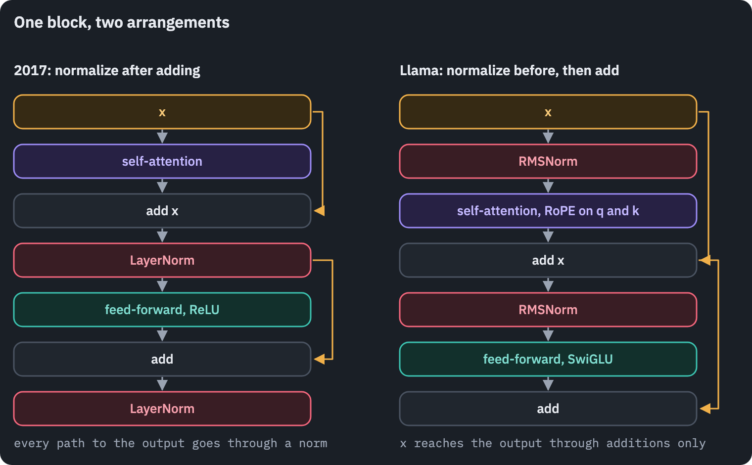
Why bother? The gradient travels the same paths backwards. In pre-norm it reaches every layer straight through the sum; in post-norm it has to pass through every norm on the way down.
Xiong et al. (2020) showed that at the start of training this leaves post-norm’s gradients largest near the output, and “using a large learning rate on those gradients makes the training unstable”.
That is what lesson 3’s warm-up was for. Pre-norm, they found, trains without one. Section 10 checks.
The history is a little funny. Five months after the paper, its authors’ own code, tensor2tensor, switched its default to pre-norm.
A comment by Noam Shazeer, one of the authors, still sits in that code: post-norm is “the published version of the transformer”, pre-norm “seems better for harder-to-learn models, so it should probably be the default”. GPT-2 moved the norm “to the input of each sub-block” in 2019, GPT-3 kept it, and Llama credits GPT-3.
One caveat that concerns us directly: Wang et al. (2019) found pre-norm slightly behind post-norm in shallow models. Ours has three layers per stack.
In code, the two arrangements differ by where one call goes. One consequence of pre-norm is easy to miss: the stream itself is never normalized, so the stack ends with one more norm of its own, before the output layer.
def residual(x, sublayer, norm, dropout, pre_norm):
    if pre_norm:
        return x + dropout(sublayer(norm(x)))  # normalize the copy, add to the stream
    return norm(x + dropout(sublayer(x)))  # 2017: add, then normalize the stream
6. RMSNorm
LayerNorm, from lesson 2, does two things to a vector: it subtracts the mean of its \(d\) numbers and divides by their standard deviation, then applies a learned scale \(\mathbf{g}\) and shift \(\mathbf{b}\). RMSNorm[5] keeps only the division, by the root mean square, and only the scale:
\[\mathrm{LayerNorm}(\mathbf{x}) = \mathbf{g} \odot \frac{\mathbf{x} - \mu}{\sqrt{\sigma^2 + \epsilon}} + \mathbf{b}, \qquad \mathrm{RMSNorm}(\mathbf{x}) = \mathbf{g} \odot \frac{\mathbf{x}}{\sqrt{\frac{1}{d} \sum_{i=1}^{d} x_i^2 + \epsilon}}.\]\(\mu\) and \(\sigma^2\) are the mean and variance of the vector’s own \(d\) numbers, \(\epsilon\) a small constant against division by zero, \(\odot\) multiplication element by element. Same vector, both norms:
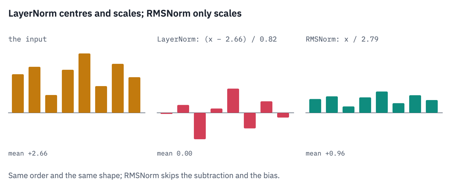
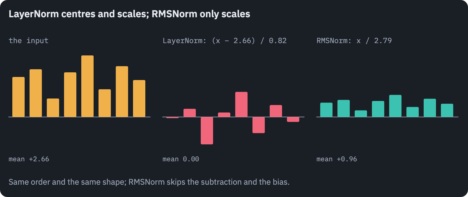
Zhang and Sennrich’s bet was that the rescaling is what makes LayerNorm work, keeping the size of the vectors in check, while “re-centering invariance in LayerNorm is dispensable”. Dropping it saves a mean and a subtraction per vector.
On a Transformer for translation they measured BLEU on a par with LayerNorm and training about 7% faster; the “7%∼64%” of their abstract comes from other models. Seven percent is modest. On a model trained for months on thousands of GPUs, modest is a lot of money.
The statistics are computed in float32 even when the rest runs in half precision: a sum of squares of a thousand numbers is exactly the kind of computation float16 gets wrong (lesson 3, section 6).
class RMSNorm(nn.Module):
    def __init__(self, d_model, eps=1e-6):
        super().__init__()
        self.eps = eps
        self.weight = nn.Parameter(torch.ones(d_model))  # g; there is no b

    def forward(self, x):
        x32 = x.float()
        mean_square = x32.pow(2).mean(dim=-1, keepdim=True)
        normed = x32 * torch.rsqrt(mean_square + self.eps)  # rsqrt: 1 / sqrt
        return (normed * self.weight).to(x.dtype)


x = torch.randn(8, 16, 256)
ours = RMSNorm(256)(x)
theirs = nn.RMSNorm(256, eps=1e-6)(x)  # PyTorch's own, since version 2.4
assert torch.allclose(ours, theirs, atol=1e-6)
print("RMSNorm agrees with torch.nn.RMSNorm")
RMSNorm agrees with torch.nn.RMSNorm7. SwiGLU
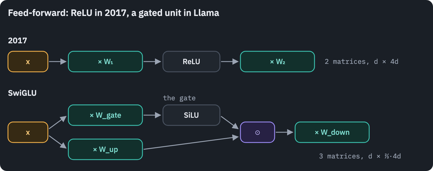
The feed-forward layer of 2017 is two matrices with a ReLU between them. SwiGLU [6] uses three: one result passes through an activation and becomes a gate that multiplies the other, element by element, before the third matrix:
\[\mathrm{FFN}_{\text{ReLU}}(x) = \max(0,\, xW_1 + b_1)\, W_2 + b_2, \qquad \mathrm{FFN}_{\text{SwiGLU}}(x) = \big(\mathrm{SiLU}(xW_{\text{gate}}) \odot xW_{\text{up}}\big)\, W_{\text{down}}.\]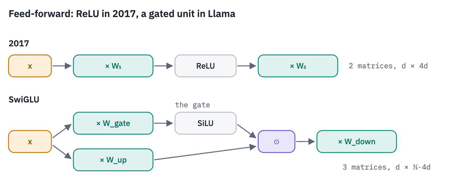
The activation is SiLU, \(\mathrm{SiLU}(z) = z \cdot \sigma(z)\), where \(\sigma\) is the logistic sigmoid; the paper calls it Swish, hence the name. Next to ReLU:
z = torch.linspace(-5, 3, 400)
fig, ax = plt.subplots(figsize=(6.4, 2.8))
ax.plot(z, torch.relu(z), color=COLORS["muted"], label="ReLU")
ax.plot(z, F.silu(z), color=COLORS["enc"], label="SiLU(z) = z·σ(z)")
ax.axhline(0, color=COLORS["line"], linewidth=0.8)
ax.set_xlabel("z")
ax.set_title("ReLU and SiLU")
ax.legend()
plt.show()
print("smallest value of SiLU:", round(F.silu(z).min().item(), 3))
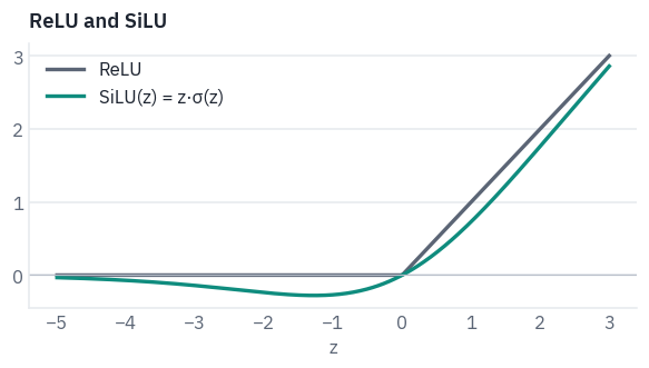
smallest value of SiLU: -0.278SiLU is ReLU with the corner rounded off: smooth everywhere, slightly negative for negative inputs, close to the identity for large ones. But the activation is the smaller change. In ReLU’s layer each hidden unit is on or off depending on one projection of the input; in SwiGLU one projection decides, smoothly, how much of another gets through.
Why that should work better, nobody can say exactly, including its author. His paper ends: “We offer no explanation as to why these architectures seem to work; we attribute their success, as all else, to divine benevolence.” It survived Narang et al.’s reimplementation, as one of the few changes that did.
Three matrices instead of two would mean more weights. To compare fairly, the hidden width shrinks to two thirds of the ReLU layer’s, as in the paper and in Llama, rounded here to a multiple of 8, which GPUs like:
class SwiGLU(nn.Module):
    def __init__(self, d_model, d_ff):
        super().__init__()
        self.w_gate = nn.Linear(d_model, d_ff, bias=False)
        self.w_up = nn.Linear(d_model, d_ff, bias=False)
        self.w_down = nn.Linear(d_ff, d_model, bias=False)

    def forward(self, x):
        return self.w_down(F.silu(self.w_gate(x)) * self.w_up(x))


class FeedForward(nn.Module):  # lesson 2's, for comparison
    def __init__(self, d_model, d_ff):
        super().__init__()
        self.linear1 = nn.Linear(d_model, d_ff)
        self.linear2 = nn.Linear(d_ff, d_model)

    def forward(self, x):
        return self.linear2(torch.relu(self.linear1(x)))


def swiglu_width(d_ff, multiple=8):
    return multiple * round(2 * d_ff / 3 / multiple)


def parameters(module):
    return sum(p.numel() for p in module.parameters())


print("ReLU, d_ff = 1024:", parameters(FeedForward(256, 1024)))
print(f"SwiGLU, d_ff = {swiglu_width(1024)}:", parameters(SwiGLU(256, swiglu_width(1024))))
ReLU, d_ff = 1024: 525568
SwiGLU, d_ff = 680: 522240
Within a percent of each other: two matrices of the full width against three of two thirds.
8. Rotary position embeddings
Lesson 2 told the model where each token stands by adding a vector of sinusoids to its embedding. The position then travels inside the token’s vector through every layer, mixed with its meaning. RoPE, rotary position embedding[7], adds nothing to the embeddings.
It acts inside attention: before the dot product, it rotates each query and each key by an angle that grows with the token’s position.
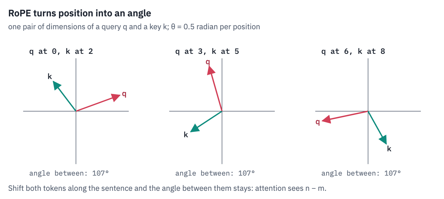
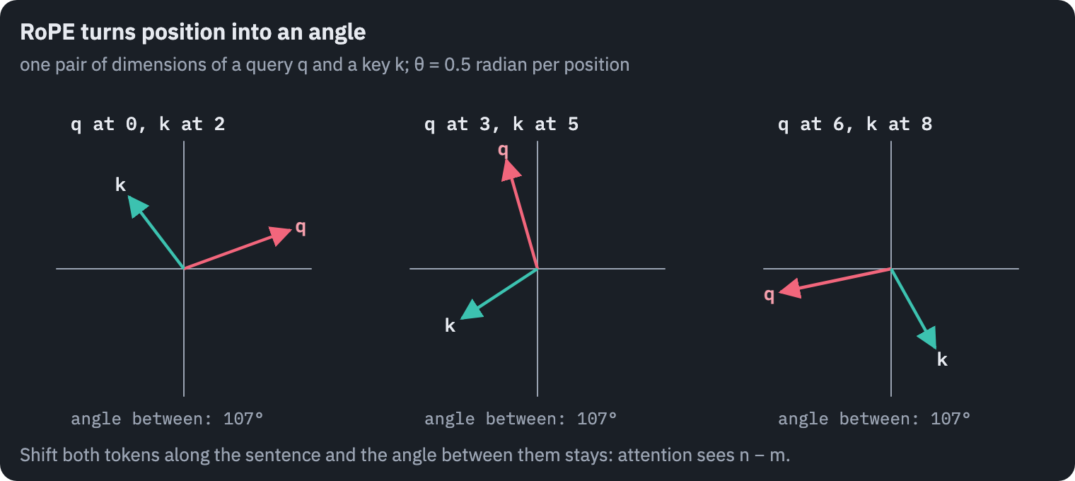
The \(d_k\) numbers of a query or a key are split into pairs, and pair \(i\) is rotated, as a point in a plane, by the angle \(m\theta_i\) for the token at position \(m\):
\[\begin{pmatrix} q'_{2i} \\ q'_{2i+1} \end{pmatrix} = \begin{pmatrix} \cos m\theta_i & -\sin m\theta_i \\ \sin m\theta_i & \cos m\theta_i \end{pmatrix} \begin{pmatrix} q_{2i} \\ q_{2i+1} \end{pmatrix}, \qquad \theta_i = b^{-2i/d_k},\quad i = 0, \dots, \tfrac{d_k}{2} - 1.\]Write \(R(\alpha)\) for the rotation by \(\alpha\). A rotation’s transpose rotates back, \(R(\alpha)^\top = R(-\alpha)\), and rotations add up, so for a query at position \(m\) and a key at position \(n\):
\[\big(R(m\theta)\,q\big)^\top \big(R(n\theta)\,k\big) = q^\top R(-m\theta) R(n\theta)\, k = q^\top R\big((n - m)\theta\big)\, k.\]The attention score depends on the positions only through \(n - m\), the distance between the two tokens. That’s a relative position, given to attention directly, which is what the sinusoids of 2017 only hoped the model would work out for itself.
Each pair turns at its own speed. With \(b = 10\,000\), the first pair advances a radian per token and the last needs tens of thousands of tokens for one turn; a full turn of pair \(i\) takes \(2\pi / \theta_i\) tokens:
def rope_angles(max_len, d_k, base=10_000):
    theta = base ** (-torch.arange(0, d_k, 2) / d_k)  # one speed per pair: (d_k / 2,)
    positions = torch.arange(max_len)
    return positions[:, None] * theta[None, :]  # the angle m·θ_i: (max_len, d_k / 2)


d_k = 256 // 4  # our heads
wavelengths = 2 * math.pi / rope_angles(2, d_k)[1]  # tokens per full turn, pair by pair
llama_wavelengths = 2 * math.pi / rope_angles(2, 128, base=llama["rope_theta"])[1]

fig, ax = plt.subplots(figsize=(6.4, 3))
label = "ours: d_k = 64, b = 10 000"
ax.plot(wavelengths, "o", color=COLORS["enc"], markersize=4, label=label)
label = f"Llama 3.1: d_k = 128, b = {llama['rope_theta']:,.0f}"
ax.plot(llama_wavelengths, ".", color=COLORS["att"], markersize=3, label=label)
ax.axhline(MAX_LEN, color=COLORS["dec"], linestyle=(0, (3, 3)), linewidth=1)
ax.text(40, MAX_LEN * 1.4, "our longest training sentence", fontsize=9, color=COLORS["dec"])
ax.set_yscale("log")
ax.set_xlabel("pair i")
ax.set_ylabel("tokens per full turn")
ax.set_title("Every pair rotates at its own speed")
ax.legend(fontsize=9)
plt.show()
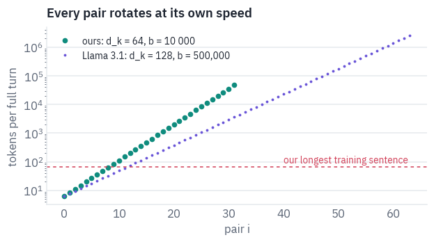
Over our longest sentence, the fast pairs turn many times and the slow ones hardly start: together they tell near positions apart and far ones too, like the hands of a clock. Llama’s base, fifty times larger, slows every pair down further, so that positions far apart in a context of many thousands of tokens still get different angles.
The rotation in code works on all pairs at once: the even and the odd numbers of every query or key, each pair with its own angle.
def apply_rope(x, angles):
    # x: (B, H, T, d_k); angles: (T, d_k / 2), one angle per position and pair
    cos, sin = angles.cos().to(x.dtype), angles.sin().to(x.dtype)
    even, odd = x[..., 0::2], x[..., 1::2]
    rotated = torch.empty_like(x)
    rotated[..., 0::2] = even * cos - odd * sin
    rotated[..., 1::2] = even * sin + odd * cos
    return rotated
Two checks. The derivation promised that only \(n - m\) matters: shift a query and a key by the same number of positions and every score must stay. And Meta’s original Llama code computes the same rotation another way, with complex numbers: a pair \((a, b)\) is the number \(a + ib\), and multiplying it by \(e^{im\theta_i}\) rotates it by \(m\theta_i\). Ours must agree with that too.
q, k = torch.randn(1, 1, 30, 64), torch.randn(1, 1, 30, 64)
angles = rope_angles(100, 64)
scores_here = apply_rope(q, angles[:30]) @ apply_rope(k, angles[:30]).transpose(-1, -2)
scores_later = apply_rope(q, angles[7:37]) @ apply_rope(k, angles[7:37]).transpose(-1, -2)
assert torch.allclose(scores_here, scores_later, atol=1e-4)

# Meta's way (llama/model.py): pairs as complex numbers, times e^(i·angle)
q_complex = torch.view_as_complex(q.reshape(1, 1, 30, 32, 2))
rotation = torch.polar(torch.ones(30, 32), angles[:30])  # e^(i·m·θ_i)
meta = torch.view_as_real(q_complex * rotation).flatten(-2)
assert torch.allclose(meta, apply_rope(q, angles[:30]), atol=1e-6)
print("shift-invariant, and equal to the complex-number version")
shift-invariant, and equal to the complex-number versionWhere does RoPE go in a translator? Llama has self-attention only. Our encoder’s self-attention compares English tokens with English tokens, the decoder’s Russian with Russian, and there RoPE does what it does in Llama.
Cross-attention compares a Russian position with an English one, in two different sentences, and the difference between their positions means nothing in particular. So cross-attention gets no rotation and learns the alignment between the languages from content alone, as lesson 3’s attention maps showed it can.
9. The model, with every change behind a switch
Now the pieces go into one model with three switches: norm (post for 2017, pre for pre-norm with LayerNorm, rms for pre-norm with RMSNorm), ffn (relu or swiglu) and pos (sinusoidal or rope).
The names of the parameters are lesson 2’s, so that the 2017 setting can load lesson 3’s trained weights, the strongest check that nothing else changed.
Attention first. It takes the RoPE angles for its queries and keys (none in cross-attention), uses the fused function, and accepts a cache, which section 11 explains.
class Attention(nn.Module):
    def __init__(self, d_model, n_heads, fused=True):
        super().__init__()
        self.n_heads, self.d_k, self.fused = n_heads, d_model // n_heads, fused
        self.w_q = nn.Linear(d_model, d_model)
        self.w_k = nn.Linear(d_model, d_model)
        self.w_v = nn.Linear(d_model, d_model)
        self.w_o = nn.Linear(d_model, d_model)

    def split_heads(self, x):
        batch, length, _ = x.shape
        return x.view(batch, length, self.n_heads, self.d_k).transpose(1, 2)

    def keys_values(self, x, angles=None):
        k, v = self.split_heads(self.w_k(x)), self.split_heads(self.w_v(x))
        if angles is not None:
            k = apply_rope(k, angles)
        return k, v

    def forward(self, x_query, x_key_value, mask, angles=None, cache=None):
        q = self.split_heads(self.w_q(x_query))
        if angles is not None:
            q = apply_rope(q, angles)
        if cache is not None and cache.get("fixed"):  # cross-attention, once (section 11)
            k, v = cache["k"], cache["v"]
        else:
            k, v = self.keys_values(x_key_value, angles)
            if cache is not None:  # self-attention: the cached past plus the new ones
                if "k" in cache:
                    k = torch.cat([cache["k"], k], dim=2)
                    v = torch.cat([cache["v"], v], dim=2)
                cache["k"], cache["v"] = k, v
        if self.fused:
            out = F.scaled_dot_product_attention(q, k, v, attn_mask=mask)
        else:
            out = attention(q, k, v, mask)
        batch, _, length, _ = out.shape
        return self.w_o(out.transpose(1, 2).reshape(batch, length, -1))
A block, encoder or decoder: the decoder’s has cross-attention in the middle. Every sublayer goes through residual of section 5.
class Block(nn.Module):
    def __init__(self, d_model, n_heads, d_ff, dropout, cross, setup):
        super().__init__()
        self.pre_norm = setup["norm"] != "post"
        Norm = RMSNorm if setup["norm"] == "rms" else nn.LayerNorm
        fused = setup.get("fused", True)
        self.self_attention = Attention(d_model, n_heads, fused)
        self.cross_attention = Attention(d_model, n_heads, fused) if cross else None
        if setup["ffn"] == "swiglu":
            self.feed_forward = SwiGLU(d_model, swiglu_width(d_ff))
        else:
            self.feed_forward = FeedForward(d_model, d_ff)
        self.norm1, self.norm2 = Norm(d_model), Norm(d_model)
        if cross:
            self.norm3 = Norm(d_model)
        self.dropout = nn.Dropout(dropout)

    def forward(self, x, mask, angles, memory=None, memory_mask=None, cache=None):
        def sub(x, sublayer, norm):
            return residual(x, sublayer, norm, self.dropout, self.pre_norm)

        own = cache["self"] if cache else None
        x = sub(x, lambda h: self.self_attention(h, h, mask, angles, own), self.norm1)
        if self.cross_attention is None:  # an encoder block
            return sub(x, self.feed_forward, self.norm2)
        other = cache["cross"] if cache else None

        def cross(h):
            return self.cross_attention(h, memory, memory_mask, cache=other)

        x = sub(x, cross, self.norm2)
        return sub(x, self.feed_forward, self.norm3)
And the model. With RoPE there are no sinusoids to add, only a table of angles; with pre-norm each stack ends with its own norm. Everything else is lesson 2’s.
class Seq2Seq(nn.Module):
    def __init__(self, setup, vocab_size, d_model=256, n_heads=4, d_ff=1024, n_layers=3,
                 dropout=0.1, pad_id=0, max_len=256):
        super().__init__()
        self.setup, self.d_model, self.pad_id = setup, d_model, pad_id
        self.embedding = nn.Embedding(vocab_size, d_model)
        nn.init.normal_(self.embedding.weight, mean=0.0, std=d_model**-0.5)
        if setup["pos"] == "sinusoidal":
            self.register_buffer("pe", positional_encoding(max_len, d_model))
        else:
            self.register_buffer("angles", rope_angles(max_len, d_model // n_heads))
        args = (d_model, n_heads, d_ff, dropout)
        self.encoder = nn.ModuleList([Block(*args, False, setup) for _ in range(n_layers)])
        self.decoder = nn.ModuleList([Block(*args, True, setup) for _ in range(n_layers)])
        self.dropout = nn.Dropout(dropout)
        if setup["norm"] != "post":  # pre-norm: one more norm at the end of each stack
            Norm = RMSNorm if setup["norm"] == "rms" else nn.LayerNorm
            self.encoder_norm, self.decoder_norm = Norm(d_model), Norm(d_model)

    def embed(self, ids, start=0):
        x = self.embedding(ids) * math.sqrt(self.d_model)
        if self.setup["pos"] == "sinusoidal":
            x = x + self.pe[start : start + ids.shape[1]]
        return self.dropout(x)

    def rope(self, length, start=0):
        if self.setup["pos"] != "rope":
            return None
        return self.angles[start : start + length]

    def encode(self, src):
        mask = (src != self.pad_id)[:, None, None, :]  # (B, 1, 1, S): which keys are real
        x = self.embed(src)
        for layer in self.encoder:
            x = layer(x, mask, self.rope(src.shape[1]))
        return self.encoder_norm(x) if self.setup["norm"] != "post" else x

    def decode(self, tgt, memory, src):
        length = tgt.shape[1]
        causal = torch.ones(length, length, dtype=torch.bool, device=tgt.device).tril()
        mask = causal[None, None] & (tgt != self.pad_id)[:, None, None, :]
        memory_mask = (src != self.pad_id)[:, None, None, :]
        x = self.embed(tgt)
        for layer in self.decoder:
            x = layer(x, mask, self.rope(length), memory, memory_mask)
        if self.setup["norm"] != "post":
            x = self.decoder_norm(x)
        return x @ self.embedding.weight.T

    def forward(self, src, tgt):
        return self.decode(tgt, self.encode(src), src)
The five rungs of the ladder:
VARIANTS = {
    "2017": {"norm": "post", "ffn": "relu", "pos": "sinusoidal"},
    "+ pre-norm": {"norm": "pre", "ffn": "relu", "pos": "sinusoidal"},
    "+ RMSNorm": {"norm": "rms", "ffn": "relu", "pos": "sinusoidal"},
    "+ SwiGLU": {"norm": "rms", "ffn": "swiglu", "pos": "sinusoidal"},
    "+ RoPE": {"norm": "rms", "ffn": "swiglu", "pos": "rope"},
}


def new_model(setup, seed=SEED):
    torch.manual_seed(seed)  # the same starting weights wherever the shapes allow
    return Seq2Seq(setup, VOCAB_SIZE, pad_id=PAD).to(device)


rows = []
for name, setup in VARIANTS.items():
    rows.append({"model": name, "parameters": parameters(new_model(setup))})
table(pd.DataFrame(rows))
| model | parameters |
|---|---|
| 2017 | 9,625,600 |
| + pre-norm | 9,626,624 |
| + RMSNorm | 9,622,272 |
| + SwiGLU | 9,602,304 |
| + RoPE | 9,602,304 |
Pre-norm adds two norms, RMSNorm drops their shifts, SwiGLU stays within a percent of ReLU, and RoPE removes nothing that was learned, because the sinusoids never were. The ladder compares designs, not sizes.
The strongest check: the 2017 setting must be lesson 3’s model. Load lesson 3’s trained weights into it and compare the outputs on a batch of validation sentences.
MODEL_REPO = "xmarva/tfs-transformer-en-ru"
with open(hf_hub_download(MODEL_REPO, "config.json")) as f:
    CONFIG = json.load(f)
lesson3 = Transformer(**CONFIG).to(device).eval()
lesson3.load_state_dict(load_file(hf_hub_download(MODEL_REPO, "model.safetensors")))

rebuilt = new_model(VARIANTS["2017"]).eval()
rebuilt.load_state_dict(lesson3.state_dict())  # every name must match, nothing left over
src_ids, tgt_in, _ = (t.to(device) for t in valid_batches[0])
with torch.no_grad():
    difference = (lesson3(src_ids, tgt_in) - rebuilt(src_ids, tgt_in)).abs().max().item()
assert difference < 1e-3
print("largest difference from lesson 3's model:", difference)
largest difference from lesson 3's model: 1.1444091796875e-05The difference is rounding: the fused function adds the same numbers in a different order. So the first rung of the ladder is lesson 3’s model itself, and every other rung differs from it by its switches and nothing else.
What fused attention buys in training, measured on the 2017 model: a few dozen steps each way, after a few to warm the GPU up.
def ms_per_step(model, n_steps=30):
    optimizer = training.adam(model)
    run = dict(pad_id=PAD, device=device)
    training.train_steps(model, optimizer, train_batches, lambda step: 1e-4, 5, **run)
    if device == "cuda":
        torch.cuda.synchronize()
    start = time.perf_counter()
    training.train_steps(model, optimizer, train_batches, lambda step: 1e-4, n_steps, **run)
    if device == "cuda":
        torch.cuda.synchronize()
    return (time.perf_counter() - start) / n_steps * 1000


TIMING_STEPS = 30 if not SMOKE else 2
manual = ms_per_step(new_model({**VARIANTS["2017"], "fused": False}), TIMING_STEPS)
fused = ms_per_step(new_model(VARIANTS["2017"]), TIMING_STEPS)
print(f"lesson 2's attention: {manual:.0f} ms per step; fused: {fused:.0f} ms per step")
lesson 2's attention: 65 ms per step; fused: 62 ms per stepOn our sentences, a dozen tokens long, fused attention saves only a little: the \(T \times T\) matrices are tiny, and the time goes elsewhere. FlashAttention’s gains grow with the length of the sequence, which is why every model with a long context uses it. For us it’s a small gain for free, with the same results.
10. The ablation ladder
First, warm-up
Section 5 claimed that pre-norm trains without a warm-up. Lesson 3 showed what happens to the 2017 design without one: train for 1,500 steps at a high constant learning rate and the loss gets stuck. Repeat that experiment with the pre-norm model next to it:
PEAK = 3e-3  # lesson 3's experiment
EXPERIMENT_STEPS = 1_500 if not SMOKE else 10
experiments = [
    ("2017, no warm-up", VARIANTS["2017"], lambda step: PEAK),
    ("2017, warm-up over 1 000 steps", VARIANTS["2017"],
     lambda step: PEAK * min(1.0, step / 1_000)),
    ("pre-norm, no warm-up", VARIANTS["+ pre-norm"], lambda step: PEAK),
]
curves = {}
for name, setup, schedule in experiments:
    random.seed(SEED)
    model = new_model(setup)
    optimizer = training.adam(model)
    run = dict(pad_id=PAD, device=device)
    curves[name] = training.train_steps(model, optimizer, train_batches, schedule,
                                        EXPERIMENT_STEPS, **run)

fig, ax = plt.subplots(figsize=(6.4, 3.2))
colors = [COLORS["dec"], COLORS["muted"], COLORS["enc"]]
for (name, losses), color in zip(curves.items(), colors):
    smooth = pd.Series(losses).rolling(25, min_periods=1).mean()
    ax.plot(smooth, color=color, label=name)
ax.set_xlabel("step")
ax.set_ylabel("training loss (smoothed)")
ax.set_title("A high learning rate from the first step")
ax.legend(fontsize=9)
plt.show()
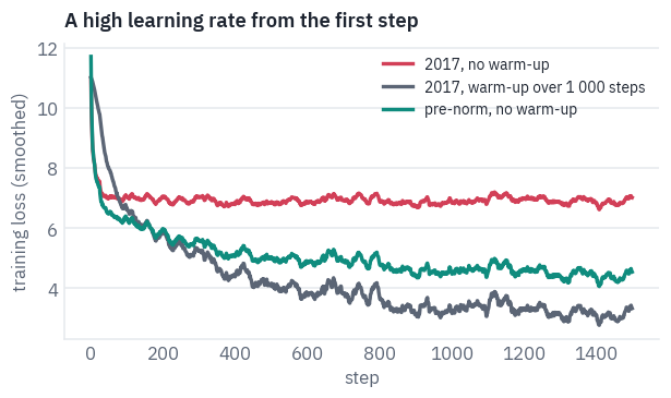
Without a warm-up, the 2017 model gets stuck, as in lesson 3. The pre-norm model doesn’t: its loss falls from the first steps at full speed.
It is behind the 2017 model with a warm-up, though. Pre-norm removes the need for a warm-up, not the benefit of one.
Five models, one budget
Every model now trains for the same number of steps on the same batches, with the same schedule and seed. Lesson 3’s schedule warms up for almost five epochs, longer than these runs last, so they use a shorter one: the same peak learning rate as lesson 3, reached in 1,000 steps, then the same \(1/\sqrt{t}\) decay.
Five epochs per model is short of the twenty of lesson 3. That is the usual bargain of an ablation: many models trained briefly rather than one trained well, on the assumption that what helps early keeps helping, which section 12 checks for the final model.
ABLATION_EPOCHS = 5 if not SMOKE else 1
ABLATION_PEAK, ABLATION_WARMUP = 1e-3, 1_000


def ablation_schedule(step):
    return ABLATION_PEAK * min(step / ABLATION_WARMUP, math.sqrt(ABLATION_WARMUP / step))


def train_model(setup, epochs, schedule, seed=SEED, checkpoint=None):
    random.seed(seed)
    model = new_model(setup, seed)
    optimizer = training.adam(model)
    history, done, best = [], 0, float("inf")
    start = time.perf_counter()
    for epoch in range(1, epochs + 1):
        losses = training.train_steps(model, optimizer, train_batches, schedule,
                                      len(train_batches), pad_id=PAD, first_step=done + 1,
                                      device=device)
        done += len(losses)
        loss = training.validation_loss(model, valid_batches, pad_id=PAD, device=device)
        minutes = (time.perf_counter() - start) / 60
        history.append({"epoch": epoch, "validation loss": loss, "minutes": minutes})
        if checkpoint is not None and loss < best:  # keep the best weights
            best = loss
            save_file(model.state_dict(), checkpoint)
    return model, history
Six runs: the five rungs and the 2017 model again with another seed. The difference between the two 2017 runs is what chance alone does to the numbers, and any change smaller than that hasn’t shown anything. This is the long cell of the lesson.
RUNS = [(name, setup, SEED) for name, setup in VARIANTS.items()]
RUNS.append(("2017, another seed", VARIANTS["2017"], SEED + 1))

ladder_models, ladder_history = {}, {}
for name, setup, seed in RUNS:
    model, history = train_model(setup, ABLATION_EPOCHS, ablation_schedule, seed)
    ladder_models[name], ladder_history[name] = model, history
    last = history[-1]
    loss, minutes = round(last["validation loss"], 3), round(last["minutes"], 1)
    print(name, "| validation loss", loss, "|", minutes, "min")
2017 | validation loss 1.309 | 4.4 min
+ pre-norm | validation loss 1.352 | 4.4 min
+ RMSNorm | validation loss 1.351 | 5.1 min
+ SwiGLU | validation loss 1.296 | 5.3 min
+ RoPE | validation loss 1.269 | 5.7 min
2017, another seed | validation loss 1.337 | 4.4 minfig, ax = plt.subplots(figsize=(6.4, 3.4))
colors = [COLORS["muted"], COLORS["data"], COLORS["dec"], COLORS["enc"], COLORS["att"],
COLORS["line"]]
for (name, history), color in zip(ladder_history.items(), colors):
epochs = [record["epoch"] for record in history]
losses = [record["validation loss"] for record in history]
style = (0, (3, 3)) if "seed" in name else "-"
ax.plot(epochs, losses, marker="o", markersize=3, color=color, linestyle=style,
label=name)
ax.set_xlabel("epoch")
ax.set_ylabel("validation loss")
ax.set_title("Six models, one budget")
ax.legend(fontsize=8)
plt.show()
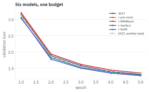
Six curves, falling together; the differences at the end are small. Mind the minutes in the printout too: RMSNorm, SwiGLU and RoPE each made training a little slower.
Our RMSNorm and RoPE are several small operations each, and every one is a separate trip through the GPU’s memory, the very thing fused attention avoids. Production implementations fuse them as well.
The validation loss is a loss, not a translation. Translate a sample of 5,000 test pairs with each model, greedy as in lesson 4’s comparison, and score them with lesson 4’s metrics: BLEU and chrF from sacreBLEU, which lesson 4 checked ours against, and COMET from tfs.comet, lesson 4’s forward pass. Check the package against the official scores lesson 4 used, first:
comet = Comet(device)
# (source, translation, reference, score from unbabel-comet 2.2.7), as in lesson 4
PACKAGE_SCORES = [
    ("The researcher said she was exhausted.", "Исследователь сказал, что она устала.",
     "Исследовательница сказала, что вымоталась.", 0.873125),
    ("Tom forgot to lock the door.", "Tom forgot to lock the door.",
     "Том забыл запереть дверь.", 0.614086),
]
for source, translation, reference, theirs in PACKAGE_SCORES:
    ours = comet.score([source], [translation], [reference])[0]
    assert abs(ours - theirs) < 1e-4
print("tfs.comet gives the package's scores")
tfs.comet gives the package's scoressample = test.sample(min(5_000, len(test)), random_state=SEED).reset_index(drop=True)
rows = []
for name, model in ladder_models.items():
hypotheses = decoding.greedy(model, tokenizer, list(sample.en))
sample[name] = hypotheses
sample[f"COMET {name}"] = comet.score(sample.en, hypotheses, sample.ru)
rows.append(
{
"model": name,
"validation loss": ladder_history[name][-1]["validation loss"],
"BLEU": sacrebleu.corpus_bleu(hypotheses, [list(sample.ru)]).score,
"chrF": sacrebleu.corpus_chrf(hypotheses, [list(sample.ru)]).score,
"COMET": sample[f"COMET {name}"].mean(),
}
)
ladder_scores = pd.DataFrame(rows)
table(ladder_scores, digits=3)
| model | validation loss | BLEU | chrF | COMET |
|---|---|---|---|---|
| 2017 | 1.309 | 34.831 | 53.130 | 0.820 |
| + pre-norm | 1.352 | 34.206 | 52.647 | 0.813 |
| + RMSNorm | 1.351 | 33.921 | 52.530 | 0.813 |
| + SwiGLU | 1.296 | 35.136 | 53.796 | 0.823 |
| + RoPE | 1.269 | 35.718 | 54.302 | 0.826 |
| 2017, another seed | 1.337 | 34.232 | 53.185 | 0.827 |
Read the last row first: the 2017 design trained again with another seed. Nothing changed but chance, and the two runs differ in COMET by about as much as neighbouring rungs do. They don’t even agree on the direction: the second run has the higher loss and the higher COMET.
Keep that in mind for the rest of the table. Pre-norm raised the loss and lowered COMET, Wang et al.’s caveat about shallow models; RMSNorm left both where they were, which is the whole of its promise; SwiGLU and RoPE lowered the loss and raised COMET.
Which of the differences are real? Lesson 4’s paired bootstrap, on COMET, which lesson 4 found the least noisy per sentence: every model against the 2017 model, on the same thousand resampled test sets.
def bootstrap_against(name, baseline="2017", draws=1_000):
    rng = np.random.default_rng(SEED)
    a = sample[f"COMET {name}"].to_numpy()
    b = sample[f"COMET {baseline}"].to_numpy()
    differences = []
    for _ in range(draws):
        rows_drawn = rng.integers(0, len(sample), size=len(sample))  # with replacement
        differences.append(a[rows_drawn].mean() - b[rows_drawn].mean())
    return np.array(differences)


rows = []
for name in ladder_models:
    if name == "2017":
        continue
    differences = bootstrap_against(name)
    low, high = np.percentile(differences, [2.5, 97.5])
    rows.append({"model − 2017": name, "COMET difference": differences.mean(),
                 "95% of draws from": low, "to": high,
                 "better in": f"{(differences > 0).mean():.0%}"})
table(pd.DataFrame(rows), digits=4)
| model − 2017 | COMET difference | 95% of draws from | to | better in |
|---|---|---|---|---|
| + pre-norm | -0.0070 | -0.0102 | -0.0036 | 0% |
| + RMSNorm | -0.0071 | -0.0103 | -0.0039 | 0% |
| + SwiGLU | 0.0035 | -0.0001 | 0.0071 | 97% |
| + RoPE | 0.0065 | 0.0031 | 0.0098 | 100% |
| 2017, another seed | 0.0069 | 0.0037 | 0.0104 | 100% |
The bootstrap is sure of almost every row, including the one that can’t mean anything: it finds the second run of the 2017 design better than the first in every draw, by about as much as the RoPE rung.
The bootstrap isn’t wrong. It resamples the test sentences and keeps the trained models fixed, so it answers a narrower question: would these trained models change places on another test set?
Whether another training run would land in the same place is a different question, and a different seed is enough to change the answer: other starting weights, the batches in another order.
The only way to measure that is to train again. The course trained three more seeds of the 2017 design and four of the last rung with this lesson’s code (seed_runs.py, next to this notebook) and published the scores. With this notebook’s own runs, that makes five runs of each:
SEED_RUNS = "xmarva/tfs-seed-runs-en-ru"
path = hf_hub_download(SEED_RUNS, "data/runs.parquet", repo_type="dataset")
seed_runs = pd.read_parquet(path)
columns = ["setup", "seed", "validation loss", "COMET"]

ours = ladder_scores.set_index("model")
here = []  # this notebook's own runs: (setup, seed, name in the ladder)
here.append(("2017", SEED, "2017"))
here.append(("2017", SEED + 1, "2017, another seed"))
here.append(("+ RoPE", SEED, "+ RoPE"))
rows = []
for setup, seed, name in here:
    rows.append({"setup": setup, "seed": seed, "COMET": ours.loc[name, "COMET"],
                 "validation loss": ours.loc[name, "validation loss"]})
other_seeds = seed_runs[seed_runs.epochs == 5][columns]
short_runs = pd.concat([pd.DataFrame(rows), other_seeds], ignore_index=True)

designs = [("2017", COLORS["muted"]), ("+ RoPE", COLORS["att"])]
fig, axes = plt.subplots(1, 2, figsize=(6.4, 2.9))
for ax, metric in zip(axes, ["COMET", "validation loss"]):
    for k, (setup, color) in enumerate(designs):
        values = short_runs[short_runs.setup == setup][metric].to_numpy()
        offsets = np.linspace(-0.12, 0.12, len(values))  # close values stay visible
        ax.scatter(k + offsets, values, color=color, s=30, zorder=3)
    ax.set_xticks([0, 1], ["2017", "all four changes"])
    ax.set_xlim(-0.6, 1.6)
axes[0].set_title("COMET, five runs of each design")
axes[1].set_title("validation loss")
plt.show()

def design(setup):
    return "2017" if setup == "2017" else "all four changes"


rows = []
for setup, runs in short_runs.groupby("setup", sort=False):
    losses = runs["validation loss"]
    rows.append({"design": design(setup), "runs": len(runs),
                 "COMET from": runs.COMET.min(), "to": runs.COMET.max(),
                 "validation loss from": losses.min(), "to ": losses.max()})
table(pd.DataFrame(rows), digits=4)
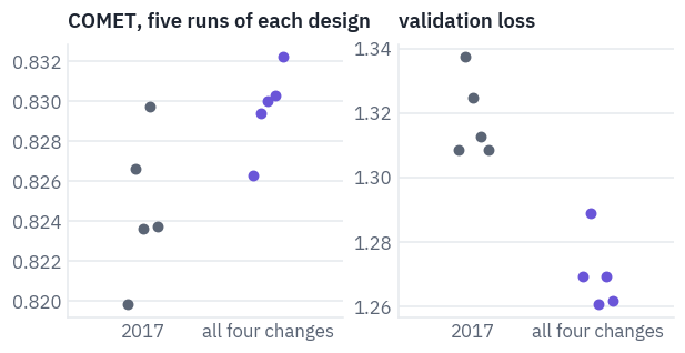
| design | runs | COMET from | to | validation loss from | to |
|---|---|---|---|---|---|
| 2017 | 5 | 0.8198 | 0.8297 | 1.3085 | 1.3374 |
| all four changes | 5 | 0.8263 | 0.8322 | 1.2605 | 1.2888 |
Five runs of the same design spread over about a hundredth of COMET, as far as the largest step of the ladder. One run per change can’t rank pre-norm, RMSNorm, SwiGLU and RoPE by COMET on five thousand sentences, however sure the bootstrap is.
The validation loss is steadier: every run of the last rung is below every run of the 2017 design. So the ladder’s overall claim holds, on the loss: all four changes together train to a lower loss in five epochs.
The single rungs are less certain. Pre-norm’s and SwiGLU’s moves in the loss are larger than the spread between seeds, RoPE’s is about as large, RMSNorm’s is nothing.
One run per change and a confident table is an easy way to fool yourself, and the way out costs compute and nothing else.
Why keep pre-norm? Because this ladder measures quality after five epochs, and pre-norm’s gift is stability: a model that trains without a warm-up and survives higher learning rates. That matters more as models get deeper, and lesson 6, which tunes the learning rate, measures how much it is worth to us.
11. A KV cache
One more change that every real model makes, and this one is about using a model rather than training it. Decoding writes one token at a time, and lesson 3’s decoder recomputes the whole prefix at every step: at step \(t\) it projects all \(t\) tokens to keys and values again, although only the newest one is new.
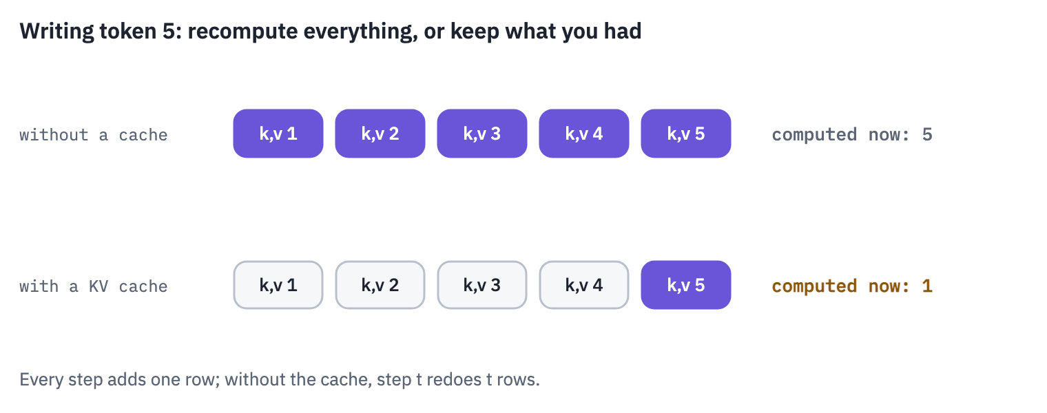
A KV cache keeps every layer’s keys and values from the previous steps, so that a step feeds the decoder only the newest token. The causal mask isn’t needed any more: the one new query may look at every key in the cache, which all belong to earlier positions.
The cross-attention’s keys and values come from the encoder’s output, which doesn’t change while a sentence is translated, so they are computed once per sentence.
RoPE makes this easy: a key is rotated by its own position once, when it enters the cache, and never touched again. With added sinusoids the same holds, since the position went in with the embedding.
The cache costs memory, and that is where section 1’s grouped-query attention comes in: every layer keeps a key and a value per key/value head for every token written so far. From Llama’s config:
def cache_bytes_per_token(layers, kv_heads, head_dim, bytes_per_number=2):
    return 2 * layers * kv_heads * head_dim * bytes_per_number  # a key and a value


head_dim = llama["hidden_size"] // llama["num_attention_heads"]
layers = llama["num_hidden_layers"]
with_gqa = cache_bytes_per_token(layers, llama["num_key_value_heads"], head_dim)
without_gqa = cache_bytes_per_token(layers, llama["num_attention_heads"], head_dim)
print(f"Llama 3.1 8B in bfloat16: {with_gqa / 1024:.0f} KiB per token")
print(f"with a key/value head per query head: {without_gqa / 1024:.0f} KiB per token")
print(f"a full context of 128K tokens: {with_gqa * 128 * 1024 / 2**30:.0f} GiB")
Llama 3.1 8B in bfloat16: 128 KiB per token
with a key/value head per query head: 512 KiB per token
a full context of 128K tokens: 16 GiB
Gigabytes for the cache of a single long conversation, on top of the weights: this is why grouped-query attention spread so fast. Our model, with four heads and sentences of a dozen tokens, keeps a few kilobytes per token.
Attention already handles a cache dictionary (section 9). The step function gives each decoder layer one, and greedy decoding runs on it:
def decode_step(model, token, memory, src, caches, position):
    memory_mask = (src != model.pad_id)[:, None, None, :]
    x = model.embed(token, start=position)  # (B, 1, d_model): only the newest token
    angles = model.rope(1, start=position)
    for layer, cache in zip(model.decoder, caches):
        x = layer(x, None, angles, memory, memory_mask, cache)  # no mask: all keys are past
    if model.setup["norm"] != "post":
        x = model.decoder_norm(x)
    return (x @ model.embedding.weight.T)[:, -1]


@torch.no_grad()
def greedy_cached(model, sentences, max_tokens=60, batch_size=256):
    model.eval()
    order = sorted(range(len(sentences)), key=lambda i: len(sentences[i]))
    translations = [None] * len(sentences)
    for start in range(0, len(order), batch_size):
        rows_here = order[start : start + batch_size]
        ids = [tokenizer.encode(sentences[i]).ids for i in rows_here]
        src = training.pad_batch(ids, PAD).to(device)
        memory = model.encode(src)
        caches = []
        for layer in model.decoder:  # cross-attention: keys and values once per sentence
            k, v = layer.cross_attention.keys_values(memory)
            caches.append({"self": {}, "cross": {"fixed": True, "k": k, "v": v}})
        token = torch.full((len(rows_here), 1), BOS, device=device)
        written = []
        done = torch.zeros(len(rows_here), dtype=torch.bool, device=device)
        for position in range(max_tokens):
            scores = decode_step(model, token, memory, src, caches, position)
            next_ids = scores.argmax(dim=-1)
            next_ids[done] = PAD  # a finished sentence only collects padding
            written.append(next_ids)
            done |= next_ids == EOS
            if done.all():
                break
            token = next_ids[:, None]
        written = torch.stack(written, dim=1).tolist()
        for row, i in zip(written, rows_here):
            ids = []
            for token_id in row:
                if token_id in (EOS, PAD):
                    break
                ids.append(token_id)
            translations[i] = tokenizer.decode(ids)
    return translations
The cache must not change a single translation. Check that on the sample of section 10 with the “+ RoPE” model, and time both ways:
model = ladder_models["+ RoPE"]
sentences = list(dict.fromkeys(sample.en))

start = time.perf_counter()
plain = decoding.greedy(model, tokenizer, sentences)
plain_seconds = time.perf_counter() - start
start = time.perf_counter()
cached = greedy_cached(model, sentences)
cached_seconds = time.perf_counter() - start

same = sum(a == b for a, b in zip(plain, cached))
print(f"same translation: {same} of {len(sentences)}")
print(f"without a cache: {plain_seconds:.1f} s, with: {cached_seconds:.1f} s")
same translation: 4796 of 4796
without a cache: 9.7 s, with: 2.9 s
The same translations, several times faster. And the longer the sentence, the bigger the factor: without a cache, step \(t\) recomputes \(t\) positions, so a sentence of \(T\) tokens costs about \(T^2/2\) of them; with the cache it costs \(T\).
12. The final model
Over five seeds, all four changes together train to a lower loss than the 2017 design in five epochs. Does that hold over a full training run? Train the last rung, all four changes, the way lesson 3 trained its model.
The recipe is lesson 3’s, to the letter: twenty epochs, the 2017 schedule with its 4,000 warm-up steps, the weights of the epoch with the lowest validation loss. The architecture is the only thing changed on purpose; the starting weights differ too, as between any two runs.
FINAL = VARIANTS["+ RoPE"]
FINAL_EPOCHS = 20 if not SMOKE else 1
CHECKPOINT = WORK_DIR / "llama-style.safetensors"

final, final_history = train_model(FINAL, FINAL_EPOCHS, training.paper_schedule,
                                   checkpoint=str(CHECKPOINT))
final.load_state_dict(load_file(CHECKPOINT, device=device))
final.eval()
best = min(record["validation loss"] for record in final_history)
lesson3_loss = training.validation_loss(lesson3, valid_batches, pad_id=PAD, device=device)
print("best validation loss:", round(best, 3))
print("lesson 3's model:", round(lesson3_loss, 3))
best validation loss: 1.028
lesson 3's model: 1.063
Lower than lesson 3’s model, with the same data, the same budget and the same recipe.
Now both models on the whole test set, with lesson 3’s beam search (four beams), all three metrics, and the paired bootstrap on the differences:
sentences = list(dict.fromkeys(test.en))
outputs = {
    "lesson 3": dict(zip(sentences, decoding.beam_search(lesson3, tokenizer, sentences))),
    "this lesson": dict(zip(sentences, decoding.beam_search(final, tokenizer, sentences))),
}
rows = []
for name, translations in outputs.items():
    test[name] = test.en.map(translations)
    test[f"COMET {name}"] = comet.score(test.en, test[name], test.ru)
    rows.append(
        {
            "model": name,
            "BLEU": sacrebleu.corpus_bleu(list(test[name]), [list(test.ru)]).score,
            "chrF": sacrebleu.corpus_chrf(list(test[name]), [list(test.ru)]).score,
            "COMET": test[f"COMET {name}"].mean(),
        }
    )
table(pd.DataFrame(rows), digits=3)
| model | BLEU | chrF | COMET |
|---|---|---|---|
| lesson 3 | 40.840 | 59.267 | 0.875 |
| this lesson | 41.540 | 59.896 | 0.883 |
rng = np.random.default_rng(SEED)
a = test["COMET this lesson"].to_numpy()
b = test["COMET lesson 3"].to_numpy()
differences = []
for _ in range(1_000):
    rows_drawn = rng.integers(0, len(test), size=len(test))
    differences.append(a[rows_drawn].mean() - b[rows_drawn].mean())
low, high = np.percentile(differences, [2.5, 97.5])
print(f"COMET, this lesson − lesson 3: {np.mean(differences):+.4f}")
print(f"95% of the draws between {low:+.4f} and {high:+.4f}")
COMET, this lesson − lesson 3: +0.0073
95% of the draws between +0.0063 and +0.0083
Ahead on every metric, and in every bootstrap draw. But section 10 showed what the bootstrap can’t see: lesson 3’s model is one training run of the 2017 design, and another run would have landed somewhere else. The seed runs include two more twenty-epoch runs of each design, trained with this lesson’s code and scored the same way:
rows = [{"model": "lesson 3", "design": "2017", "validation loss": lesson3_loss,
         "COMET": test["COMET lesson 3"].mean()},
        {"model": "this lesson", "design": "all four changes", "validation loss": best,
         "COMET": test["COMET this lesson"].mean()}]
for _, run in seed_runs[seed_runs.epochs == 20].iterrows():
    rows.append({"model": f"seed {run.seed}", "design": design(run.setup),
                 "validation loss": run["validation loss"], "COMET": run.COMET})
table(pd.DataFrame(rows).sort_values(["design", "COMET"]), digits=4)
| model | design | validation loss | COMET |
|---|---|---|---|
| lesson 3 | 2017 | 1.0634 | 0.8753 |
| seed 44 | 2017 | 1.0421 | 0.8784 |
| seed 43 | 2017 | 1.0378 | 0.8793 |
| seed 43 | all four changes | 1.0333 | 0.8818 |
| this lesson | all four changes | 1.0283 | 0.8827 |
| seed 44 | all four changes | 1.0271 | 0.8827 |
path = hf_hub_download(SEED_RUNS, "data/test.parquet", repo_type="dataset")
per_sentence = pd.read_parquet(path)
per_sentence = per_sentence.loc[test.index]  # the same pairs, in the order of our test set
assert (per_sentence.en.to_numpy() == test.en.to_numpy()).all()
a = test["COMET this lesson"].to_numpy()
for name in ["2017 s43, 20 epochs", "2017 s44, 20 epochs"]:
    b = per_sentence[f"COMET {name}"].to_numpy()
    rng = np.random.default_rng(SEED)
    differences = []
    for _ in range(1_000):
        rows_drawn = rng.integers(0, len(test), size=len(test))
        differences.append(a[rows_drawn].mean() - b[rows_drawn].mean())
    low, high = np.percentile(differences, [2.5, 97.5])
    seed = name.removesuffix(", 20 epochs")
    print(f"this lesson − {seed}: {np.mean(differences):+.4f}, "
          f"95% of the draws between {low:+.4f} and {high:+.4f}")
this lesson − 2017 s43: +0.0034, 95% of the draws between +0.0024 and +0.0044
this lesson − 2017 s44: +0.0042, 95% of the draws between +0.0033 and +0.0052
At twenty epochs the seeds agree far more closely than at five: the three runs of the new design are within a thousandth of COMET of each other. Lesson 3’s model is the lowest of the three 2017 runs, so part of the gap above was that run’s bad luck.
Against the 2017 runs from this lesson’s code the gain is smaller, and still there: every run of the new design is above every run of the old one. That’s the honest size of what an architecture buys when the data stays the same: a few thousandths of COMET, a fraction of the distance to opus-mt-en-ru.
Lesson 4 found where lesson 3’s model breaks: long sentences. Does the new one hold together longer?
encoded = tokenizer.encode_batch(list(test.en))
test["English tokens"] = [len(encoding.ids) for encoding in encoded]
edges = [0, 5, 8, 11, 15, 20, 30, 1000]
test["length"] = pd.cut(test["English tokens"], edges)
columns = ["COMET lesson 3", "COMET this lesson"]
by_length = test.groupby("length", observed=True)[columns].mean()

labels = []
for interval in by_length.index:
    if interval.right == edges[-1]:
        labels.append(f"over {interval.left}")
    else:
        labels.append(f"{interval.left + 1}–{interval.right}")
fig, ax = plt.subplots(figsize=(6.4, 3.2))
for column, color in zip(columns, [COLORS["muted"], COLORS["att"]]):
    name = column.removeprefix("COMET ")
    ax.plot(labels, by_length[column], marker="o", color=color, label=name)
ax.set_xlabel("length of the English sentence, tokens")
ax.set_ylabel("COMET, mean")
ax.set_title("Long sentences")
ax.legend()
plt.show()
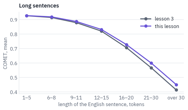
The gain isn’t spread evenly. On short sentences the two models are equal; the longer the sentence, the further ahead the new one, and long sentences are exactly where lesson 4 found lesson 3’s model breaking. It still breaks past thirty tokens, only later and less badly.
The two models’ translations of lesson 3’s sentences, side by side:
PROBES = [
    "The researcher said she was exhausted.",
    "The teacher said she was tired.",
    "Tom forgot to lock the door.",
    "We're up to our ears in debt.",
    "Australia is now considering removing humpback whales from the endangered "
    "species list because of their growing numbers.",
]
rows = []
for sentence in PROBES:
    rows.append({"English": sentence,
                 "lesson 3": decoding.beam_search(lesson3, tokenizer, [sentence])[0],
                 "this lesson": decoding.beam_search(final, tokenizer, [sentence])[0]})
table(pd.DataFrame(rows))
| English | lesson 3 | this lesson |
|---|---|---|
| The researcher said she was exhausted. | Исследователи сказали, что она измотанная. | Исследователь сказал, что она истощена. |
| The teacher said she was tired. | Учитель сказал, что она устала. | Учитель сказал, что она устала. |
| Tom forgot to lock the door. | Том забыл запереть дверь. | Том забыл запереть дверь. |
| We're up to our ears in debt. | Мы по уши в долгах. | Мы по уши в долгах. |
| Australia is now considering removing humpback whales from the endangered species list because of their growing numbers. | Австралия сейчас рассматривает колосс-похимирные шапки с корпуса из-за того, что у неё реализа того, чтобы выбрасывать чисровые чисровые чистые числы из-за того, чтобы вычивать чи | Теперь Австралия рассматривает путех чисных чисел из-за их растительных чисел. |
On short sentences the two models write the same words. The researcher sentence lost one mistake: one researcher instead of several. The noun and the verb are still masculine, the agreement lesson 2’s attention maps were about.
The long sentence about whales is still nonsense, only shorter: the first words are right, and then the model loses the thread.
13. Save and publish
The model goes to the Hub next to lesson 3’s, and its code into the course package, as tfs.modern, for the lessons that serve and deploy it. The package’s class must give exactly this lesson’s outputs:
from tfs.modern import Seq2Seq as PackageSeq2Seq

packaged = PackageSeq2Seq(FINAL, VOCAB_SIZE, pad_id=PAD).to(device).eval()
packaged.load_state_dict(final.state_dict())
with torch.no_grad():
    difference = (packaged(src_ids, tgt_in) - final(src_ids, tgt_in)).abs().max().item()
assert difference == 0
print("tfs.modern.Seq2Seq gives the same outputs")
tfs.modern.Seq2Seq gives the same outputsMODEL_DIR = WORK_DIR / "model"
MODEL_DIR.mkdir(exist_ok=True)
save_file(final.state_dict(), MODEL_DIR / "model.safetensors")
FINAL_CONFIG = {"setup": FINAL, "vocab_size": VOCAB_SIZE, "d_model": 256, "n_heads": 4,
"d_ff": 1024, "n_layers": 3, "dropout": 0.1, "pad_id": PAD}
(MODEL_DIR / "config.json").write_text(json.dumps(FINAL_CONFIG, indent=2))
print("saved:", sorted(path.name for path in MODEL_DIR.iterdir()))
saved: ['config.json', 'model.safetensors']MODEL_CARD = f"""---
license: cc-by-2.0
language: [en, ru]
tags: [translation, transformer, rope, swiglu, rmsnorm]
datasets: [xmarva/tfs-tatoeba-en-ru]
---
# A small English→Russian Transformer with Llama's changes
Built in lesson 5 of the course "Transformers: from scratch to production":
https://github.com/xmarva/transformers-from-scratch
- lesson 3's encoder-decoder (3 + 3 layers, d_model 256, 4 heads) and its recipe
- pre-norm with RMSNorm, SwiGLU feed-forward layers, rotary position embeddings
- best validation cross-entropy: {best:.3f}
```python
# pip install git+https://github.com/xmarva/transformers-from-scratch
import json
from huggingface_hub import hf_hub_download
from safetensors.torch import load_file
from tfs.modern import Seq2Seq
repo = "xmarva/tfs-transformer-en-ru-llama"
with open(hf_hub_download(repo, "config.json")) as f:
config = json.load(f)
model = Seq2Seq(**config)
model.load_state_dict(load_file(hf_hub_download(repo, "model.safetensors")))
```
"""
HUB_USER = os.environ.get("TFS_HUB_USER")
hf_token = env.secret("HF_TOKEN")
if HUB_USER and hf_token and not SMOKE:
api = HfApi(token=hf_token)
model_repo = f"{HUB_USER}/tfs-transformer-en-ru-llama"
api.create_repo(model_repo, exist_ok=True)
api.upload_folder(folder_path=str(MODEL_DIR), repo_id=model_repo)
api.upload_file(path_or_fileobj=MODEL_CARD.encode(), path_in_repo="README.md",
repo_id=model_repo)
print("published", model_repo)
else:
print("not publishing; later lessons download the course's copy:")
print("xmarva/tfs-transformer-en-ru-llama")
not publishing; later lessons download the course's copy:
xmarva/tfs-transformer-en-ru-llama
References
- Llama Team, AI @ Meta (2024). The Llama 3 Herd of Models. ↩
- Narang, S. et al. (2021). Do Transformer Modifications Transfer Across Implementations and Applications?. EMNLP. ↩
- Ainslie, J. et al. (2023). GQA: Training Generalized Multi-Query Transformer Models from Multi-Head Checkpoints. EMNLP. ↩
- Dao, T. et al. (2022). FlashAttention: Fast and Memory-Efficient Exact Attention with IO-Awareness. NeurIPS. ↩
- Zhang, B., Sennrich, R. (2019). Root Mean Square Layer Normalization. NeurIPS. ↩
- Shazeer, N. (2020). GLU Variants Improve Transformer. ↩
- Su, J. et al. (2021). RoFormer: Enhanced Transformer with Rotary Position Embedding. ↩
- Vaswani, A. et al. (2017). Attention Is All You Need. NeurIPS.
- Touvron, H. et al. (2023). LLaMA: Open and Efficient Foundation Language Models. Pre-normalization [GPT3], SwiGLU [PaLM], rotary embeddings [GPTNeo].
- Xiong, R. et al. (2020). On Layer Normalization in the Transformer Architecture. ICML.
- Wang, Q. et al. (2019). Learning Deep Transformer Models for Machine Translation. ACL.
- Radford, A. et al. (2019). Language Models are Unsupervised Multitask Learners. OpenAI. GPT-2 and pre-norm.
- Kwon, W. et al. (2023). Efficient Memory Management for Large Language Model Serving with PagedAttention. SOSP. The size of a KV cache.