Mixture of experts: why the largest LLMs use a few percent of their weights per token

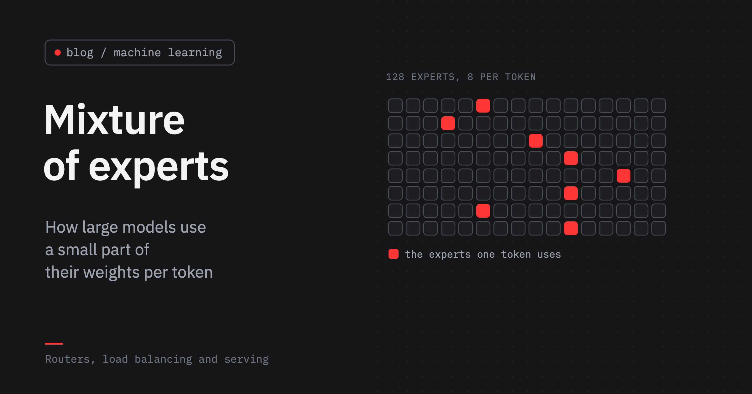
DeepSeek-V3 has 671 billion parameters and uses 37 billion of them for each token. Kimi K2 has a trillion and uses 32 billion, gpt-oss-120b uses 5.1 billion of its 117, and some names spell the arithmetic out: Qwen3-235B-A22B has 235 billion parameters, 22 billion of them active.

In every layer of these models a small router looks at the token and picks a few feed-forward networks, the experts, out of dozens or hundreds. Only those are computed. The rest of the weights wait in memory for tokens that need them.

The idea is older than the Transformer. In 1991 Jacobs, Jordan, Nowlan and Hinton described systems “composed of many separate networks, each of which learns to handle a subset of the complete set of training cases”^[1].

In 2017 Shazeer and colleagues put a layer of up to 131,072 experts between the layers of an LSTM language model^[2], and today the largest open models of DeepSeek, Qwen, Moonshot, OpenAI, Meta, Zhipu and MiniMax are all mixtures of experts.

This post builds a mixture-of-experts layer in PyTorch, trains it next to dense models of the same cost on English, Russian and Python code, and looks inside: what the router decides, why it has to be kept from playing favourites, what the experts end up specialising in, and what it takes to serve a model whose weights are mostly idle.

Where a Transformer keeps its parameters

A layer of a Transformer has two parts. Attention moves information between tokens: each token looks at the earlier ones and takes what it needs from them.

The feed-forward network then works on every token separately, with the same weights for all of them: it multiplies the token’s vector by a wide matrix, passes the result through a nonlinearity and multiplies it by a second matrix back to the original width. In modern models it is a SwiGLU network with three matrices:

Here \(x\) is the token’s vector of width \(d\), \(W_{\text{gate}}\) and \(W_{\text{up}}\) map it to a hidden width \(h\), usually three to five times \(d\), the elementwise product \(\odot\) lets one projection switch the other on and off, and \(W_{\text{down}}\) maps the result back to width \(d\).

Most of a model’s weights are in these networks. Qwen3-32B has 64 layers of width 5,120 with feed-forward networks of width 25,600, and its config gives the exact split:

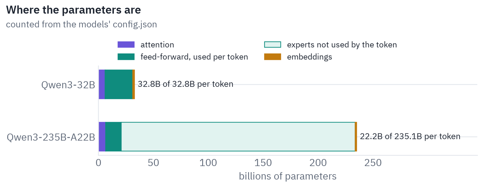
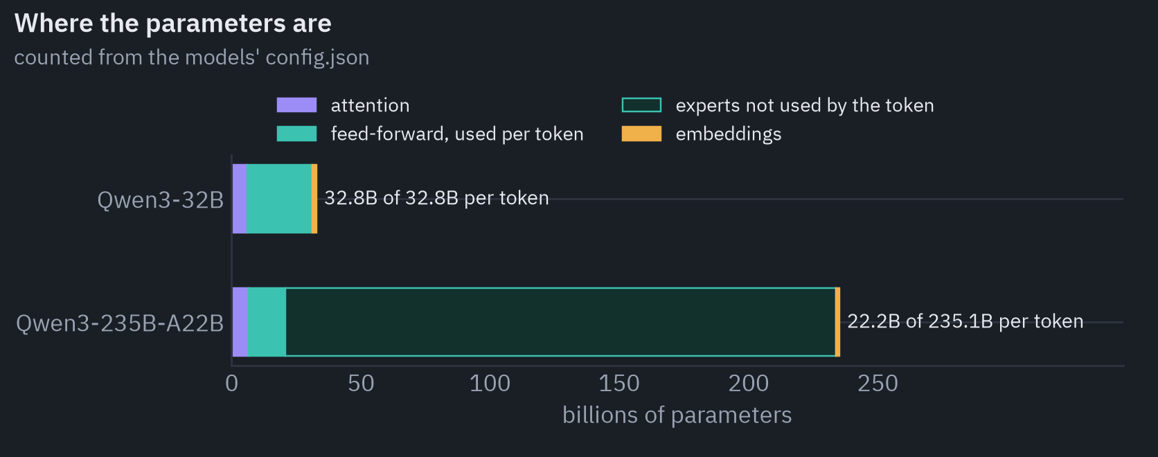
The feed-forward networks hold 25.2 billion of its 32.8 billion parameters, 77%; attention has 6.0 billion and the embeddings 1.6. Qwen3-235B-A22B, a mixture of experts of the same family, turns the picture around. Of its 235 billion parameters a token passes through 22 billion, and 213 billion, 91% of the model, are experts that this token does not use.

Every weight a token passes through costs two operations, a multiplication and an addition, so a dense model of 32 billion parameters spends about 64 billion operations on every token it reads or writes, and most of them in the feed-forward networks.

What do these networks do with so many weights? Geva and colleagues read the two matrices as a memory.

Each row of the first matrix is a key that responds to some pattern in the input, each column of the second is a value added to the output when its key responds, and the network’s output is the sum of the values whose keys fired.

In their words, feed-forward layers “operate as key-value memories, where each key correlates with textual patterns in the training examples”^[3].

A memory of 25,600 patterns of which a given token needs a few, read in full for every token, is an obvious candidate for economy. The idea of the mixture of experts is to cut it into many smaller networks and let every token use only some of them.

A layer of experts

A mixture-of-experts layer replaces the one feed-forward network with \(E\) smaller ones, the experts, and adds a router: a matrix \(W_r\) that gives every expert a score for the current token. A softmax turns the scores into probabilities, the token goes to the \(k\) experts with the highest ones, and its output is their outputs added with weights:

Term by term: \(W_r\) is an \(E \times d\) matrix, so the router is a single linear layer, tiny next to the experts. \(p_i\) is how much the router trusts expert \(i\) with this token.

\(\mathcal{T}\) is the set of the \(k\) chosen experts; the others are not computed at all, which is the whole point. The weights are the chosen probabilities divided by their sum, so they add up to one, and each \(E_i\) is an ordinary SwiGLU network, only narrower than the dense one.

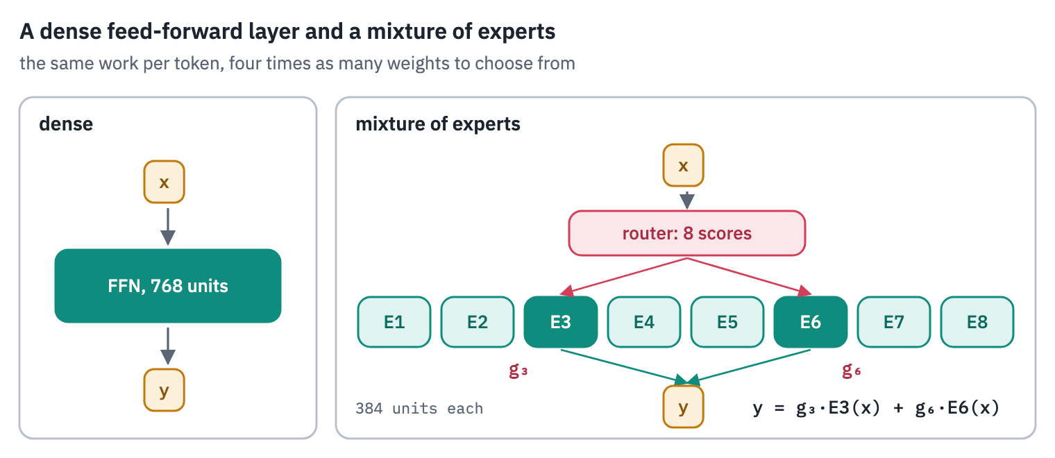
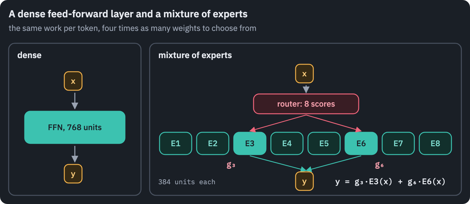
The models trained below have experts of width 384 and send every token to 2 of 8, so a token passes through 768 hidden units, as in a dense layer of width 768, while the layer holds 3,072.

Here is what the router of one of them, after training, does with the Russian word “президент” in a sentence it has not seen:

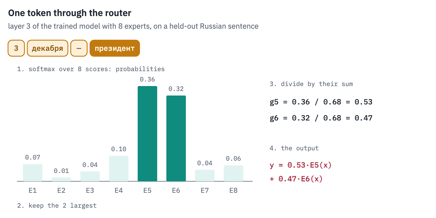
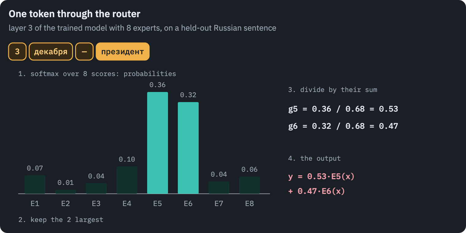
The router hesitates over this token. Experts 5 and 6 get 0.36 and 0.32 of the probability, and the other six share the remaining third, expert 4 most of it with 0.10.

The two largest probabilities are kept and divided by their sum, 0.68, which turns them into weights 0.53 and 0.47, so the token’s output is roughly half of what expert 5 computes and half of what expert 6 computes. Experts 1, 2, 3, 4, 7 and 8 never see the token at all.

The router learns with the rest of the model. Its gradient comes through the weights \(p_i / \sum_j p_j\): if expert 3’s output would have lowered the loss more than expert 7’s, the gradient raises \(p_3\) relative to \(p_7\), and the next similar token is more likely to go to expert 3.

Nothing tells the router what an expert should be good at. Specialisation, if any, appears because sending similar tokens to the same expert makes that expert better at them.

In code the layer is a loop over experts, each taking the tokens that chose it:

def moe(x, router, experts, k):
    probs = (x @ router).softmax(dim=-1)              # (tokens, experts)
    top_probs, top_experts = probs.topk(k, dim=-1)    # the k best experts of every token
    weights = top_probs / top_probs.sum(dim=-1, keepdim=True)
    out = torch.zeros_like(x)
    for e, expert in enumerate(experts):
        rows, slot = torch.nonzero(top_experts == e, as_tuple=True)   # tokens that chose e
        out[rows] += weights[rows, slot, None] * expert(x[rows])
    return out

Whether this loop is slow depends on how many tokens each expert gets. Every pass launches a few matrix products, and a GPU is efficient only when a product is large enough to keep all of its cores busy.

In training, with thousands of tokens in a batch and a handful of experts, each expert gets plenty of them. With hundreds of experts, or in decoding, where a step has one token per sequence, each expert gets a few rows, and the loop spends its time launching kernels and gathering rows instead of multiplying.

The usual remedy is to sort the token-expert pairs by expert, so that every expert’s tokens lie next to each other, and to run all the experts at once:

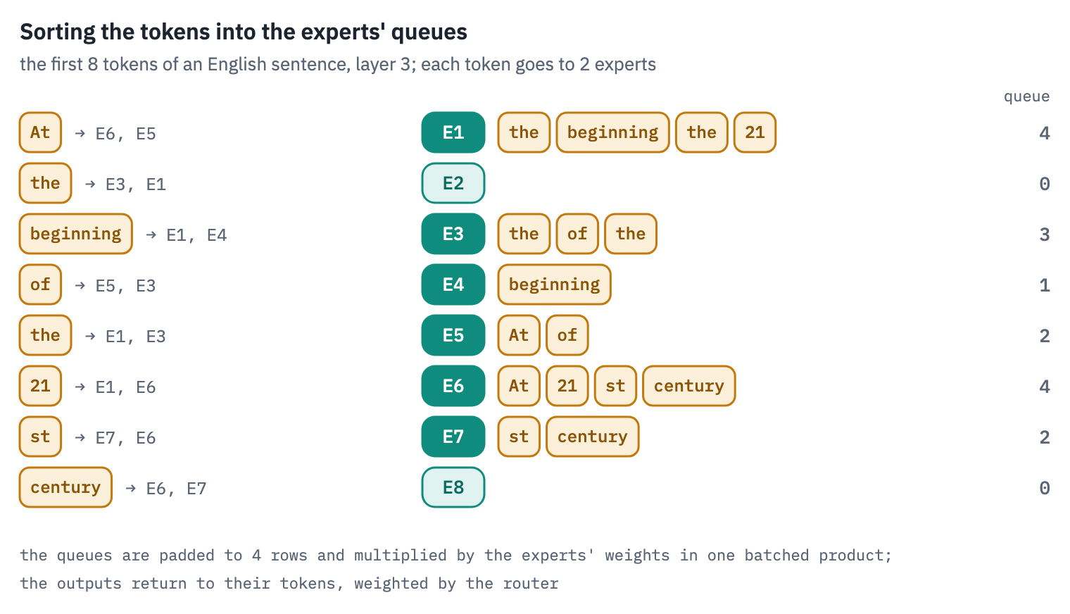
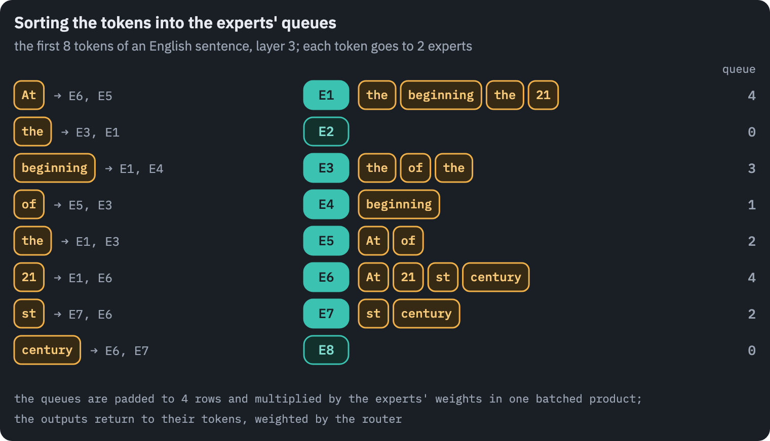
My version pads every expert’s queue to the length of the longest, rounded up to a multiple of 256 so that the GPU sees few different shapes, and multiplies all of them by the stacked expert weights in one batched product.

It agrees with a reference that runs every expert on every token and multiplies the unchosen ones by zero, to rounding error.

Production kernels avoid even the padding: MegaBlocks writes the layer as a block-sparse matrix product^[4], and DeepSeek’s DeepGEMM library has grouped products that take the experts’ tokens concatenated one after another, each expert’s segment padded only to the kernel’s block size.

Same compute, more parameters

What does a mixture buy? To see it on a small scale, I trained four models on a corpus of three kinds of text: English Wikipedia, Russian Wikipedia and the Python standard library, 8 million tokens of each, with a tokenizer of 8,192 tokens trained on the same mix (code).

All four have 6 layers of width 256 with 4 attention heads, rotary positions and RMSNorm, and differ only in the feed-forward layers.

The dense model has SwiGLU networks of width 768 and 7.2 million parameters in all. The mixture with 8 experts sends every token to 2 experts of width 384: it does the same work per token as the dense model, with 7.2 million active parameters, but holds 17.8 million.

The mixture with 32 experts cuts the same budget finer, 8 of 32 experts of width 96. The fourth model is dense with networks of width 3,072: as many parameters as the mixtures, every one of them used for every token, at about two and a half times the compute.

Each model trained three times, with different seeds, for 3,000 steps of 32 sequences of 256 tokens, about 25 million tokens, on an NVIDIA T4 on Kaggle, with the auxiliary balancing loss described below for the mixtures.

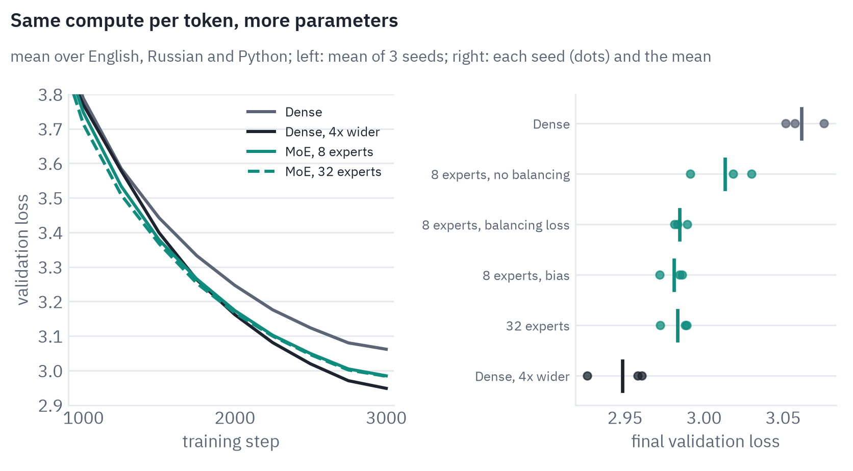
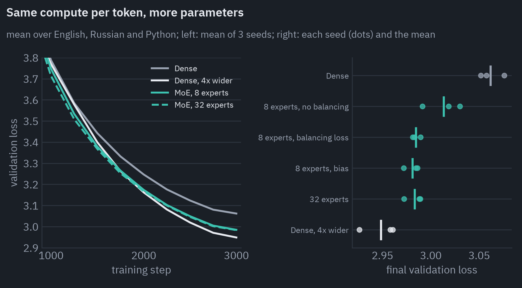
At the same compute per token, the mixture with 8 experts ends with a validation loss of 2.985 on average over the three seeds, against 3.062 for the dense model.

The three seeds of the dense model end within 0.024 of each other and those of the mixture within 0.008, so a gap of 0.077 is not noise, and the mixture is better on each kind of text: by 0.08 on English, 0.10 on Russian and 0.06 on Python.

The dense model with networks four times wider, as many parameters as the mixture and all of them working on every token, reaches 2.948, and until about step 1,750 the mixtures are even ahead of it.

The mixture gets two thirds of the way from the small dense model to the large one while computing as much as the small one.

Compute per token is not the same thing as time. Here is how long one training step takes, with the experts run by the loop shown earlier and by the sorted, batched version:

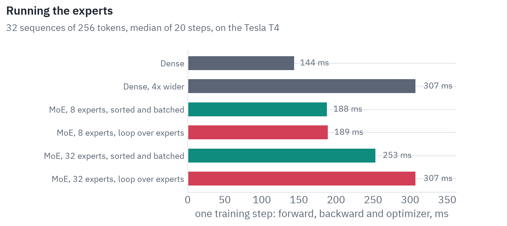
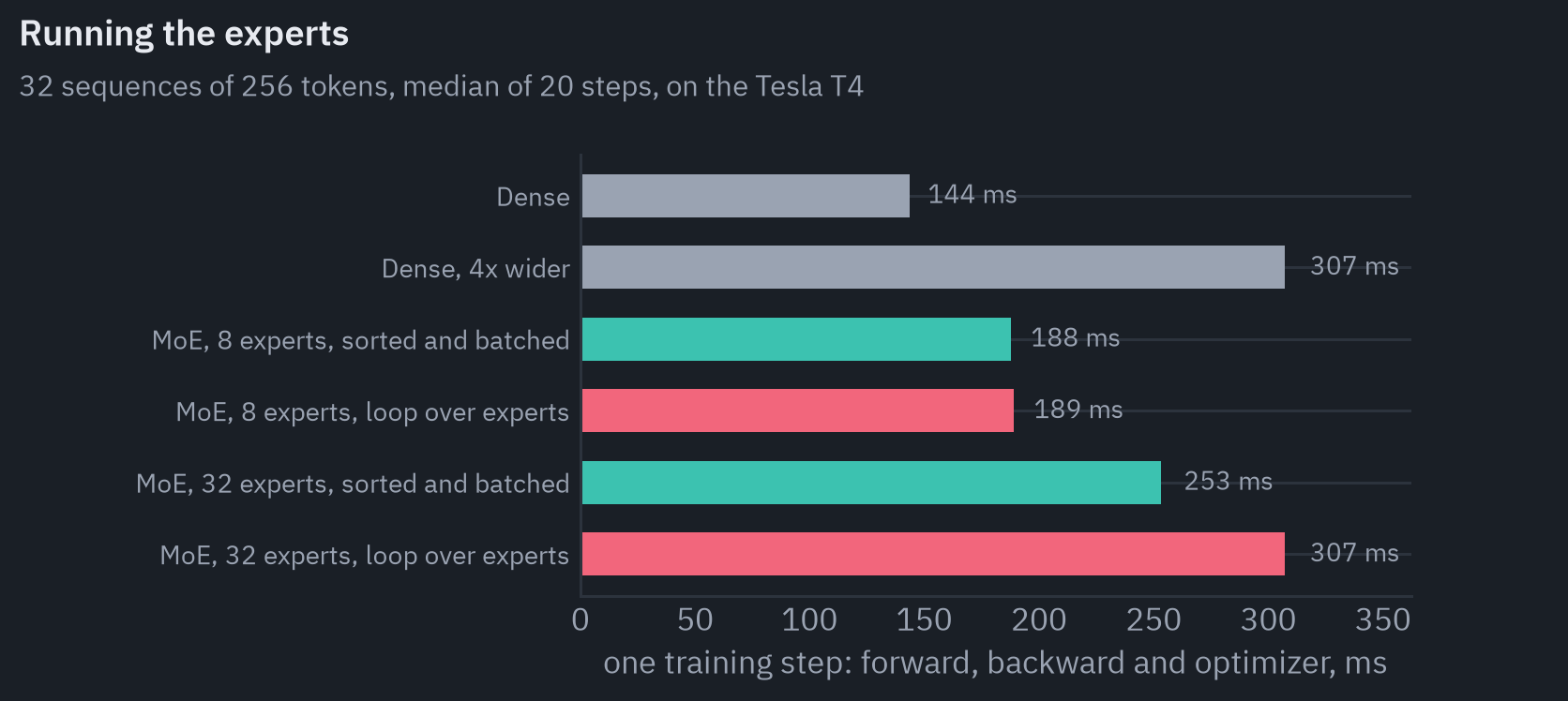
The mixture with 8 experts takes 31% longer than the dense model that does the same arithmetic, and the one with 32 experts 76% longer: routing, sorting and gathering the tokens are work that a count of multiplications doesn’t show.

The dense model with networks four times wider takes 307 milliseconds, more than twice as long as the narrow one. The loop itself turns out to be harmless here.

With 8 experts a batch of 8,192 tokens gives each expert about 2,000 of them, and the loop is as fast as the batched version, 189 against 188 milliseconds per step; with 32 narrower experts it is 21% slower.

Keeping the experts busy

Left alone, the router has a bad habit. Early in training some expert happens to be a little better than the others, the router sends it more tokens, it trains on more data and gets better still, and the router sends it even more.

The other experts get few tokens, learn little and stay unattractive. Shazeer and colleagues, who brought mixtures of experts to large networks, observed this “self-reinforcing” imbalance and countered it with an extra loss^[2].

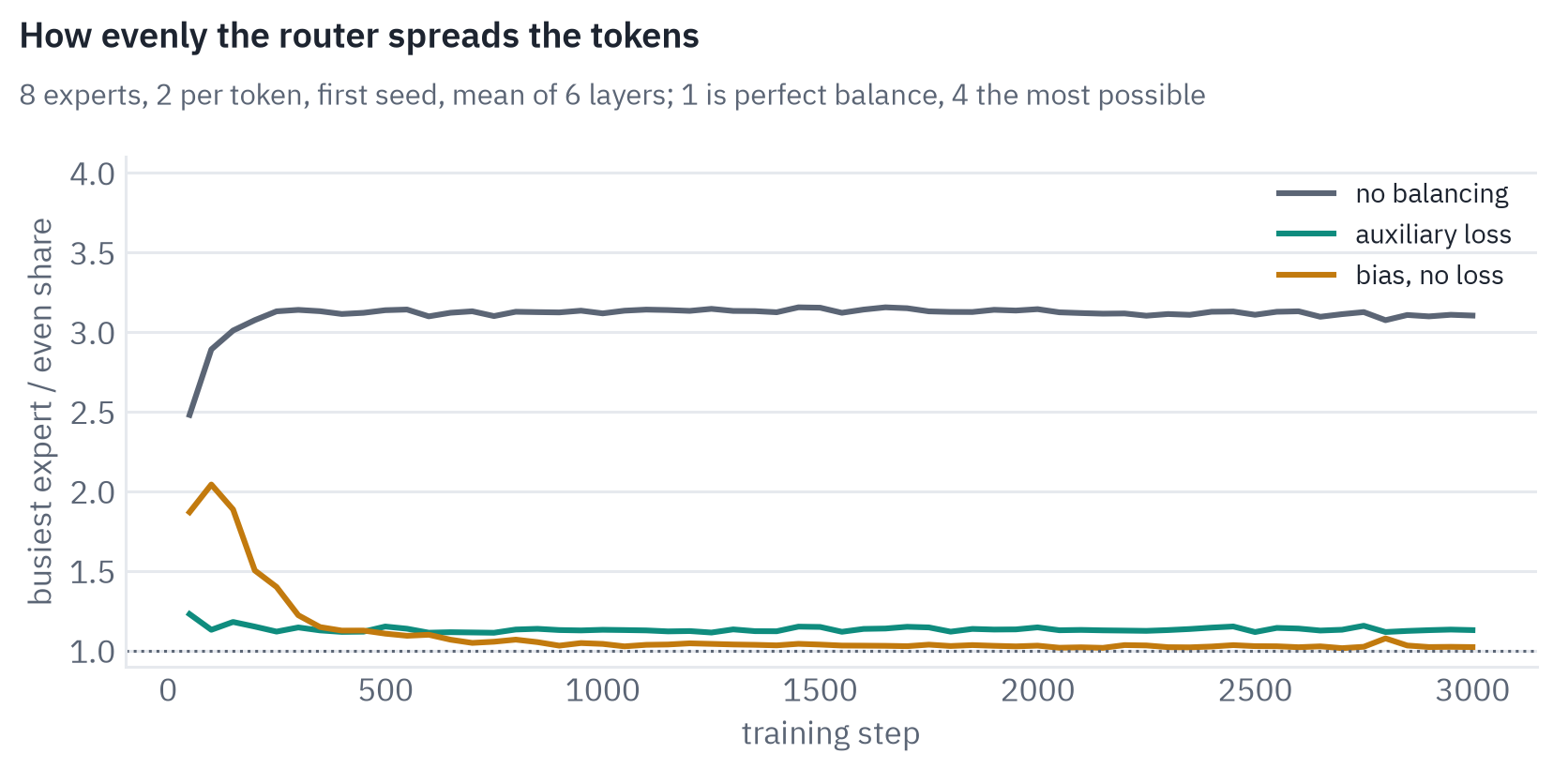
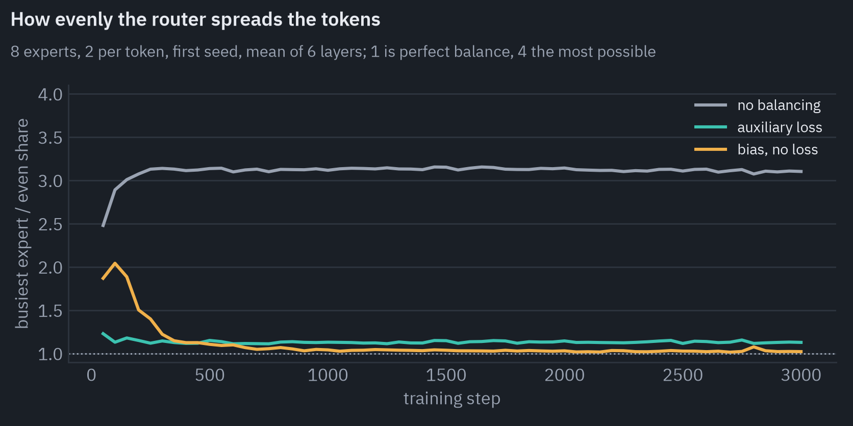
I trained the mixture with 8 experts in three versions: without any balancing, with the loss described below, and with the bias method that comes after it.

Without balancing, the busiest expert of a layer has 2.6 to 3.1 times its fair share of the tokens by step 200, and nothing ever reverses it.

On held-out text, in three of the six layers of the first of these models a single expert receives 94 to 98% of the tokens, and 9 of the 48 experts get less than a tenth of an even share. They are practically dead: their weights take memory and learn almost nothing.

With the balancing loss, the busiest expert stays at about 1.1 times an even share for the whole run. The unbalanced mixture is still better than the dense model, 3.013 against 3.062, but worse than the balanced one and less predictable: its three seeds end between 2.991 and 3.030.

The balancing loss most models use comes from the Switch Transformer^[5]. For a batch of tokens, let \(f_i\) be the share of the token-expert assignments that went to expert \(i\), and \(P_i\) the mean probability the router gave expert \(i\) over the same tokens. The loss is

added to the language modelling loss with a small weight \(\alpha\), 0.01 in the Switch Transformer and in my runs. When the router is perfectly even, \(f_i = P_i = 1/E\) and the sum times \(E\) is 1. When it favours some experts, their large \(f_i\) meet large \(P_i\) and the sum grows.

The two factors play different roles. \(f_i\) is a count of decisions, and a count has no gradient. \(P_i\) is an average of softmax outputs and has one.

So the loss pushes down the probabilities of experts that are already busy, in proportion to how busy they are, and the next tokens drift to the others. Here are both factors in two trained routers, one trained with the loss and one without:

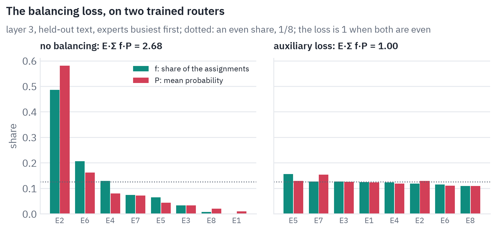
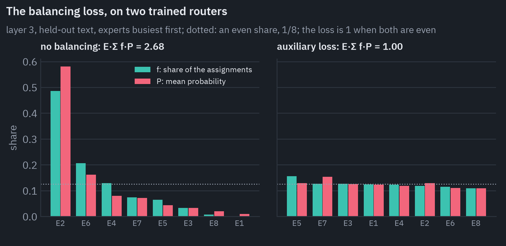
In layer 3 of the router trained without the loss, expert 2 gets 49% of the assignments, and the router’s mean probability for it is 0.58, so the router is not hesitating between experts, it is sure of its favourite.

Experts 1 and 8 get almost nothing. The loss would be 2.68 for this router. For the router trained with it, it is 1.00, and its eight experts all get between 11% and 16% of the assignments.

The extra loss has a cost: its gradient flows into the same weights as the language modelling loss and pulls them towards a goal that has nothing to do with predicting text.

Wang and colleagues at DeepSeek proposed balancing without a loss^[6], and DeepSeek-V3 uses their method^[7]. Every expert gets a bias \(b_i\) that is added to its score when the \(k\) experts are chosen, and only then:

After every training step, the bias of each expert that got fewer tokens than the average goes up by a small step \(\gamma\), and the bias of each one that got more goes down by \(\gamma\).

The biases are not learned by gradient descent and don’t touch the model’s weights; they act like a traffic controller that keeps nudging the queues until they are even. I used \(\gamma = 0.001\), the value DeepSeek-V3 used for most of its training.

The biases start at zero and move by 0.001 a step, so they need time: for the first 200 steps the busiest expert gets one and a half to two times its share.

From about step 500 on, the biases keep the load more even than the loss does, 1.02 times an even share at the end against 1.10 to 1.13.

In quality the two are the same at my scale: 2.981 with the biases and 2.985 with the loss, while the seeds of each spread over 0.014 and 0.008.

DeepSeek’s comparison on models with a billion parameters is hardly more decisive: a validation loss of 2.253 with the biases, 2.258 with a balancing loss computed over each sequence, and 2.253 with one computed over the whole batch, as mine is^[7].

A fixed budget per expert

Balancing on average is not enough when the experts sit on different GPUs. Each GPU has to reserve memory for the tokens its experts will receive before it knows how many will come, and the shapes of the arrays on an accelerator are fixed in advance.

The Switch Transformer and GShard therefore give every expert a capacity, a fixed number of slots per batch^[8]:

where \(T\) is the number of tokens in the batch, \(T k / E\) is what each expert would get with perfectly even routing, and the capacity factor \(c\), usually between 1 and 2, leaves room for unevenness.

Tokens beyond the capacity are dropped by that expert. A dropped token loses that expert’s contribution; if all its experts are full, it passes through the layer unchanged, carried only by the residual connection.

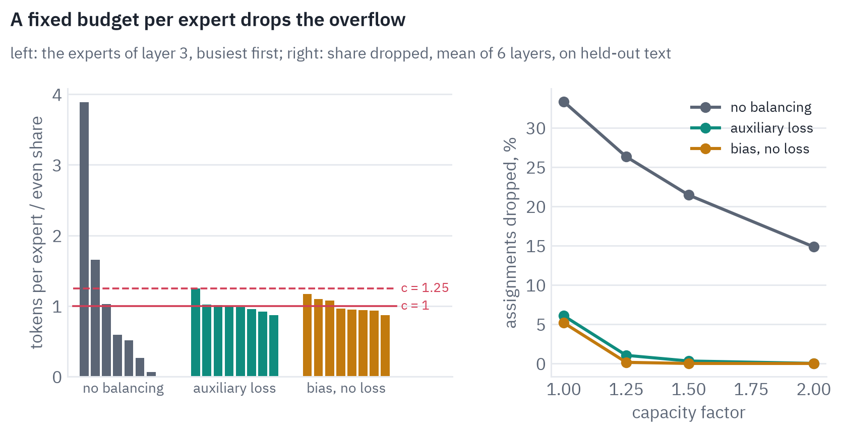
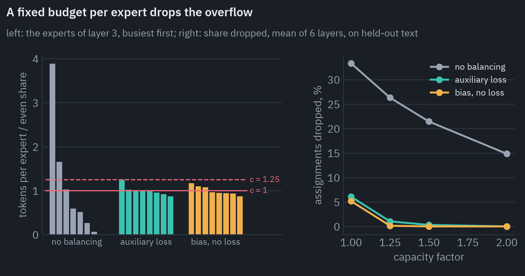
For the balanced routers a capacity factor of 1 is tight: any unevenness overflows, and 5 to 6% of the assignments are dropped. At 1.25 the share falls to 1% or less, and at 1.5 practically nothing is dropped.

The router trained without balancing is another story. At a capacity factor of 1 it drops a third of the assignments, and even at 2 it drops 15%, because its favourite experts receive nearly four times their share.

The dropped assignments cost more than their share suggests. On the held-out sequences of this analysis, the loss of the mixture with the balancing loss is 2.97 without a limit, 3.21 with 6% of the assignments dropped and 3.01 with 1%. My models were trained without a capacity limit and never learned to do without a missing expert.

A model trained with one adapts: the Switch Transformer saw “typically <1%” of tokens dropped^[5], and the ST-MoE study found that models “dropping 10-15% of tokens can perform approximately as well as models that drop <1%”^[9].

Dropping tokens is a compromise between quality and the cost of padding, and newer systems avoid it. MegaBlocks computes the experts as one block-sparse product in which every expert gets exactly the rows it was sent^[4], and DeepSeek-V3 drops no tokens in training or inference, relying on balancing to keep the load even^[7].

What the experts learn

Nobody tells an expert what to specialise in, so it is a fair question whether they specialise at all. My corpus makes it easy to see: a third English, a third Russian, a third Python, three kinds of text that differ in alphabet, vocabulary and structure. If an expert’s tokens are split evenly between the three, it has no preference.

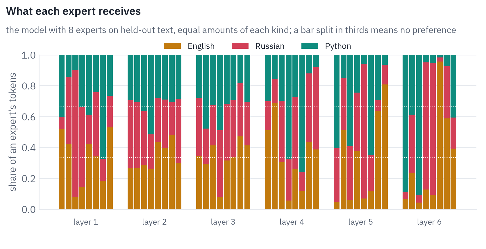
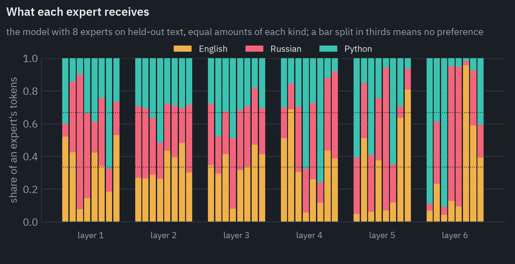
The early layers have little preference. In layers 2 and 3 no expert gets more than about half of its tokens from one kind of text, and the preference grows with depth: three experts of layer 4 lean to one kind, five of layer 5.

In layer 6 the experts have divided the languages between them. Five of the eight get 83 to 96% of their tokens from one kind of text, two from Python, two from Russian and one from English; a sixth leans to English with 59%, and two remain mixed.

The first layer stands apart from its neighbours: one of its experts gets 83% of its tokens from Russian text, another 67% from Python.

Here is the same thing token by token, on three short snippets of held-out text. Each token is coloured by the expert it goes to first:

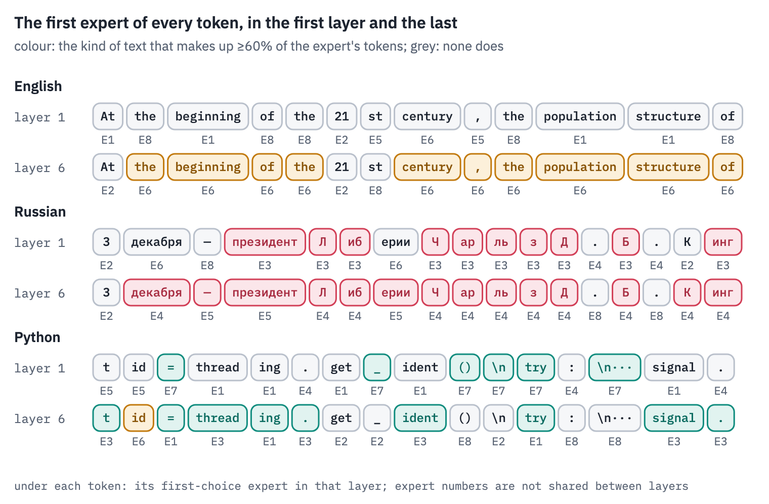
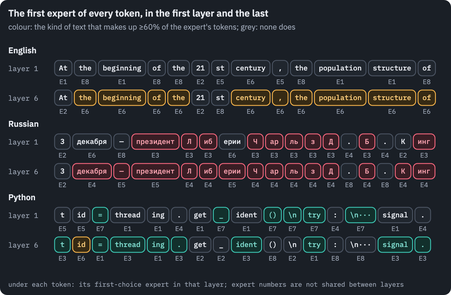
In the first layer the router sorts tokens by what they look like. Its Russian expert takes президент and most of the pieces into which the tokenizer cut the names Либерии, Чарльз and Кинг: Л, иб, Ч, ар, ль, з, Д, Б, инг.

Python’s =, _, (), try and newlines go to an expert that leans to code. English has no expert of its own in this layer at all. At this depth a token’s vector is still mostly the token itself, and the router has little else to go on.

In the last layer, 10 of the 13 English tokens, 14 of the 17 Russian ones and 9 of the 16 Python ones go to an expert of their own kind.

All the others but one go to the two mixed experts of this layer, and most of them are tokens the three kinds of text share: the numbers 3 and 21, the full stops after the initials Д. and Б., and in Python the brackets, colons, the underscore and newlines.

The last layer prepares the prediction of the next token, and what the next token can be depends first of all on the language.

Specialisation by topic, the kind people usually hope for, is much weaker in large models. Mistral looked for experts on topics in Mixtral and did not find them: “the distribution of expert assignment is very similar for ArXiv papers (written in Latex), for biology (PubMed Abstracts), and for Philosophy (PhilPapers) documents”.

What they found instead was syntax: “in code, the indentation tokens are always assigned to the same experts, particularly at the first and last layers where the hidden states are more correlated to the input and output of the model”^[10].

In OLMoE, trained from scratch with 64 small experts per layer, the specialisation is stronger: “for arXiv, which has a very specific distribution with lots of scientific text, the first expert in layer 0 is nearly 100% specialized”, and “vocabulary specialization is higher in later layers”^[11].

Languages are a case of their own. The ST-MoE study found that “experts trained on multilingual mixtures do not exhibit language specialization” and blamed the balancing: a group of tokens over which the loss was computed held only one or a few languages, so every expert had to take every language to keep the load even within the group^[9].

My batches mix all three kinds of text, and an English expert can stay busy on the English part of every batch.

Smaller experts, and one for everybody

An expert in Mixtral^[10] is as wide as the whole feed-forward network of Mistral 7B, whose architecture Mixtral otherwise shares, and a token picks 2 of 8.

DeepSeekMoE argued that this is too coarse: with only 8 experts, each has to cover a broad mix of tokens, and knowledge that all of them need is learned several times over^[12]. Their remedy has two parts.

The first is to cut every expert into \(m\) smaller ones and route each token to \(m\) times as many, which keeps the parameters and the compute the same and multiplies the number of combinations a token can choose from: in their example, top-2 of 16 experts allows 120 combinations, top-8 of 64 quarter-size experts “4,426,165,368 potential combinations”.

The second is to set aside shared experts that every token passes through, for what all tokens need, so that the routed experts can specialise.

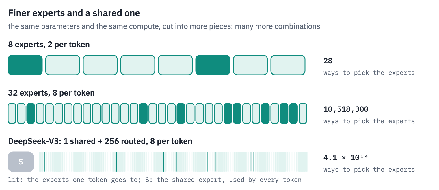
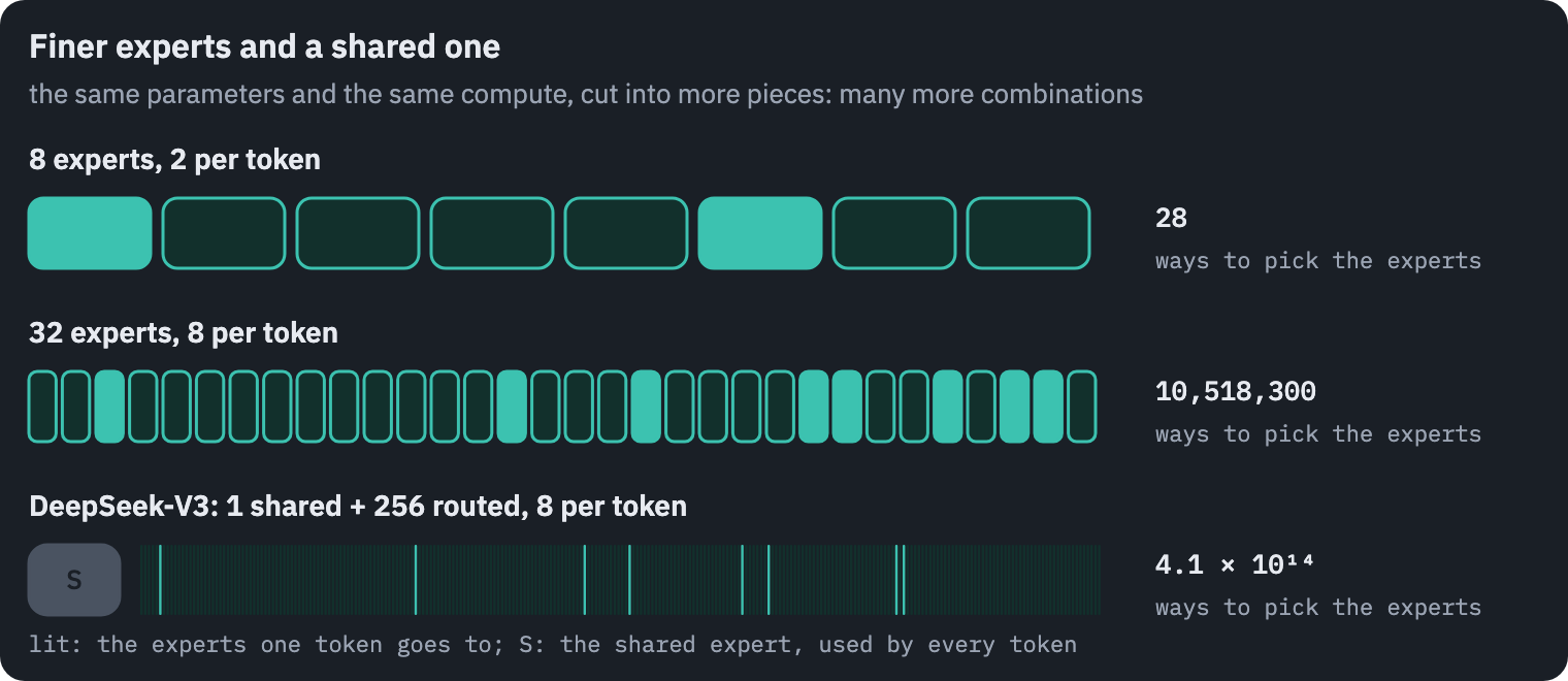
In my models the finer cut made no difference. The mixture with 32 experts ends at 2.983 and the one with 8 at 2.985, well within the spread of the seeds, and the finer one costs more time, 253 milliseconds per step against 188, because routing, sorting and gathering grow with the number of experts. It does take dropped tokens better.

With a capacity factor of 1 it loses the same 6% of its assignments as the coarse mixture, but its loss rises by 0.10 instead of 0.24: a dropped assignment takes away one of a token’s eight experts instead of one of two.

The case for finer experts was made on larger models. DeepSeekMoE’s smallest comparison is at 2 billion parameters, where “DeepSeekMoE 2B achieves comparable performance with GShard 2.9B”^[12], a hundred times the size of my models, trained on far more than my 25 million tokens.

Mixtures in real models

Here are the experts of open models as their config files describe them, in the order the models came out:

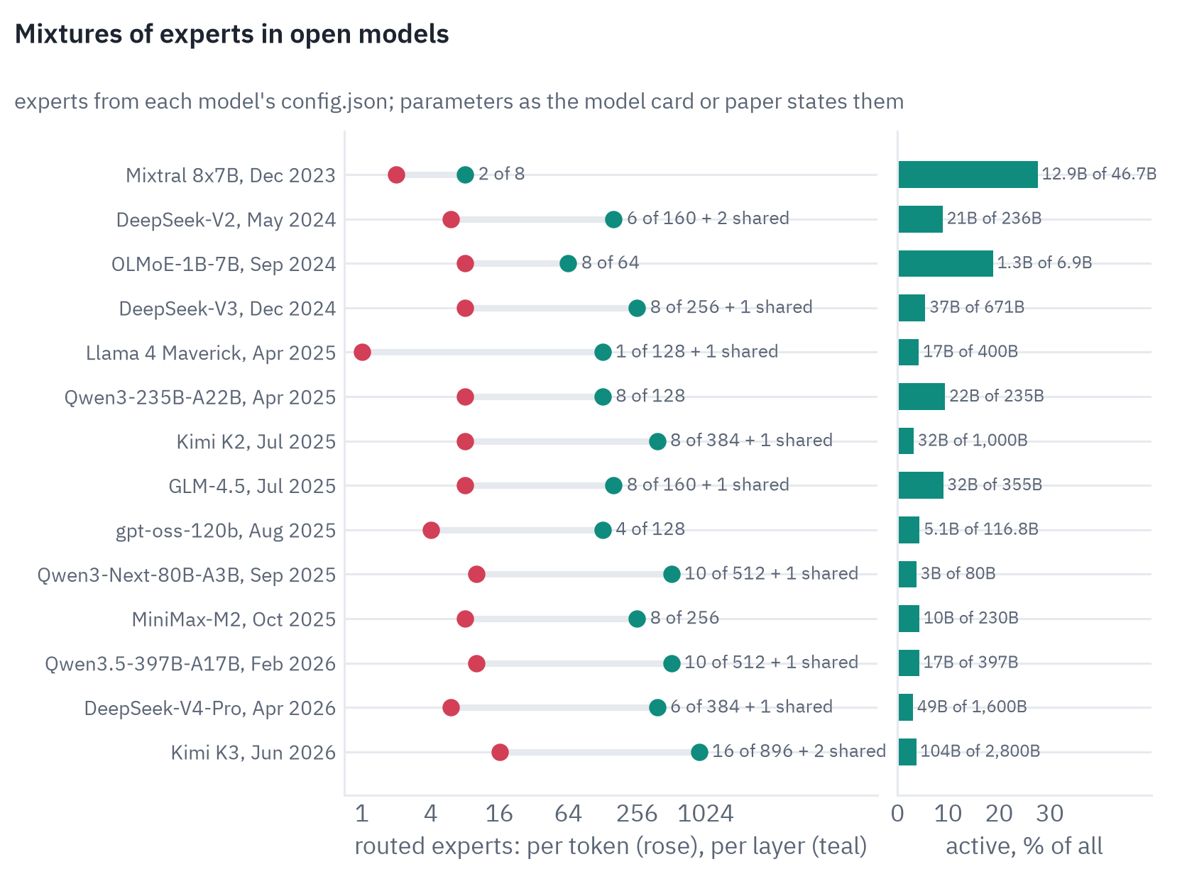
Three things changed over these two and a half years. The experts multiplied and shrank. Mixtral has 8 experts of width 14,336 per layer, DeepSeek-V3 256 of width 2,048, Kimi K3 896.

Moonshot measured the effect directly for Kimi K2: at a fixed number of active parameters, “increasing the total number of experts (i.e., increasing sparsity) consistently lowers both the training and validation loss”, and they settled on 8 of 384 as a balance between quality and the cost of the infrastructure^[13].

Krajewski and colleagues reached the same conclusion from scaling laws: setting the size of experts to match the dense feed-forward layer “is not optimal at almost any computational budget”^[14].

The active share fell accordingly, from 28% in Mixtral to 3–5% in the models of the past year. A model now holds twenty to thirty times as many parameters as it uses for a token.

The shared expert did not convince everyone. DeepSeek, Moonshot, Zhipu and the newer Qwen models use one or two; the OLMoE team found that “sharing an expert performs slightly worse” and left it out^[11], and Qwen3 also has none^[15].

Not every layer is a mixture either. DeepSeek-V3 keeps its first three layers dense, and Llama 4 Maverick alternates dense and mixture layers, with a token going to 1 of 128 routed experts plus a shared one^[16].

Serving a model that is mostly idle

The first cost of a mixture is memory. Every expert has to be at hand, because any token may need any of them, so DeepSeek-V3 needs room for all 671 billion parameters, about 671 GB at one byte per parameter in FP8, more than the 640 GB of a server with eight 80 GB GPUs.

OpenAI made gpt-oss-120b fit on one GPU by storing the experts, which hold “90+% of the total parameter count”, in a 4-bit format, MXFP4: “quantizing these to MXFP4 enables the larger model to fit on a single 80GB GPU”^[17].

A model with all its experts in memory reads only a few of them for each token. At a batch of one, the case of a chatbot on a laptop, a decoding step reads the attention weights and \(k\) experts per layer and nothing else.

Decoding is limited by how fast weights come from memory, not by arithmetic, so the step costs about as much as in a dense model of the active size.

This is why models like Qwen3-30B-A3B are popular on laptops: they need the memory of a 30-billion-parameter model but read only about 3 billion parameters per token. llama.cpp even has options to keep the experts in the computer’s main memory while the rest of the model sits on the GPU, --cpu-moe for all of them and --n-cpu-moe N for the first N layers^[18]; the GPU then holds what every token needs, and each token reads only its few experts from the slower memory.

A server decodes many conversations at once, and every conversation’s token picks its own experts. If the router spreads tokens evenly, a given expert is skipped by one token with probability \(1 - k/E\), and by all \(B\) tokens of a batch with probability \((1 - k/E)^B\). The expected share of experts a decoding step has to read is therefore

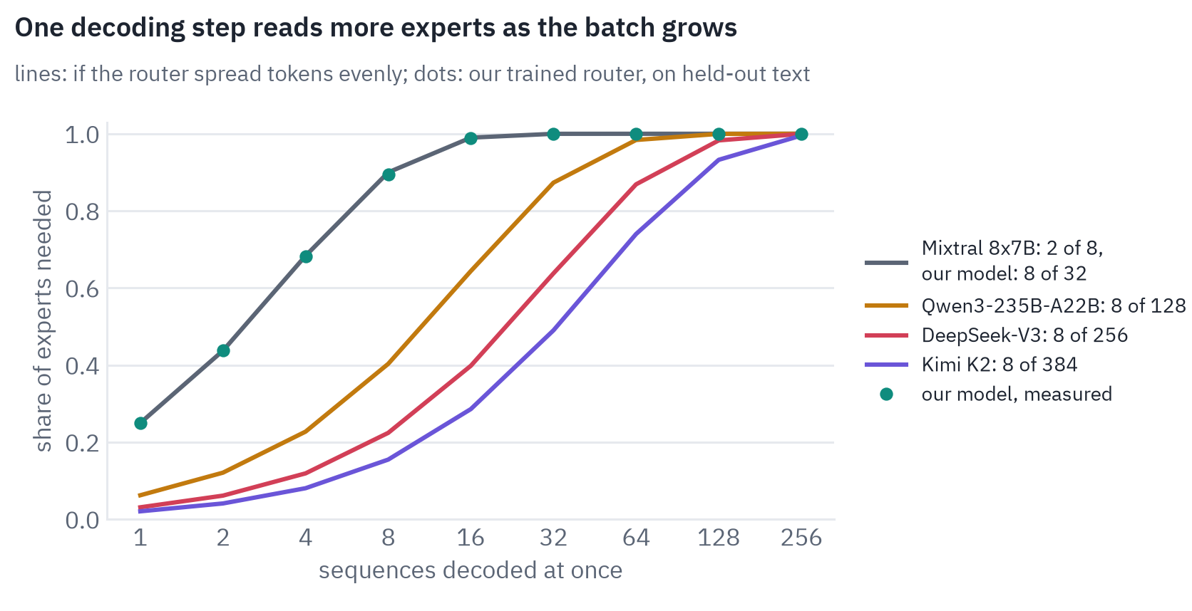
My router with 8 of 32 experts sits exactly on its curve: a decoding step needs 25% of the experts for one sequence, 90% for 8 and all of them from 32 on, as if every token picked its experts at random.

A model with a smaller share per token holds out longer. DeepSeek-V3, with 8 of 256, reads 3% of its routed experts for one sequence, 40% for 16 and 87% for 64, and from about 128 sequences on, nearly all of them.

So the saving in memory traffic that makes a mixture fast at a batch of one disappears at the batch sizes a server runs at. What remains is the saving in arithmetic: each expert multiplies only the tokens that chose it.

To turn that into speed, a server needs enough tokens per expert to keep each product efficient, and that is what expert parallelism is for: the experts are spread over many GPUs, every GPU holds a few of them, and tokens travel to their experts and back.

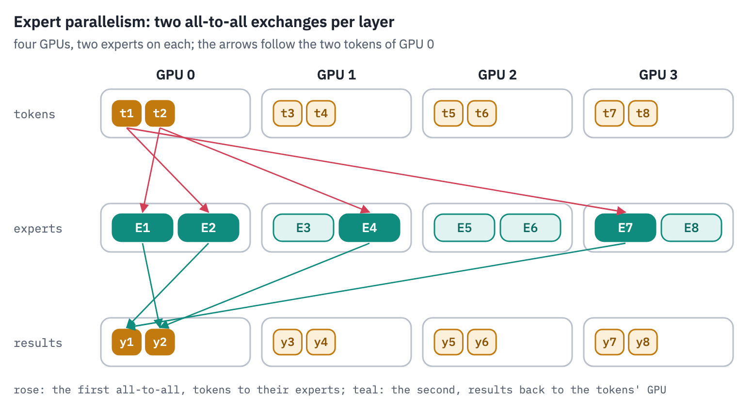
DeepSeek described its production setup for V3 and R1 in early 2025. Its reasoning is the same: “the model’s high sparsity necessitates an extremely large overall batch size. This ensures sufficient batch size per expert, enabling higher throughput and lower latency.

Large-scale cross-node EP is essential.” Reading a prompt, one deployment unit spans 4 nodes with 32-way expert parallelism; decoding, it spans 18 nodes with 144-way expert parallelism, each GPU holding 2 routed experts and the shared one, and each node of 8 GPUs writes about 14,800 tokens per second^[19].

The price is communication. Every mixture layer sends every token to other GPUs and back, twice per layer and 58 layers per token in DeepSeek-V3, and the exchange has to be hidden behind computation.

DeepSeek overlaps the communication of one batch with the computation of another and, for training, limits every token to experts on at most 4 nodes, because NVLink inside a node is about 3.2 times faster than InfiniBand between nodes^[7].

When a mixture is the right choice

A mixture of experts trades memory for compute. For a given quality it needs fewer operations per token than a dense model, and in exchange it keeps all its experts in memory and, served at scale, moves every token between GPUs and back in every layer.

The gain in compute is real and large. The Switch Transformer reached the quality of a dense T5-Base “in one-seventh the time” at the same compute per token^[5].

The gain in wall-clock time is smaller, because routing and moving tokens cost time that no operation count shows: the OLMoE team found that their mixture “reaches the performance of the dense model with ∼3× fewer tokens”, but in time “only ∼2× faster”^[11].

So the trade pays where compute is the bottleneck and memory is plentiful: training large models, and serving them to many users at once on clusters where every expert sees enough tokens to stay busy. It pays less where memory is the bottleneck or traffic is light.

The authors of GLaM, one of the first large mixtures, noted that sparse models “require a larger number of devices”, which “increases the serving cost especially when the serving traffic is low”^[20]. Fine-tuning needs care too.

In the ST-MoE study, sparse models were “prone to overfitting”: on a task with 250 training examples the sparse model did worse than the dense one, and sparse models needed their own fine-tuning settings, smaller batches and a higher learning rate^[9].

A laptop with plenty of memory and a modest processor is a case of its own. Its memory can hold all the experts, and at a batch of one each token reads only the few it needs.

References

1. Jacobs, R. A., Jordan, M. I., Nowlan, S. J., & Hinton, G. E. (1991). Adaptive mixtures of local experts. Neural Computation, 3(1), 79–87. ↩
2. Shazeer, N., Mirhoseini, A., Maziarz, K., Davis, A., Le, Q., Hinton, G., & Dean, J. (2017). Outrageously large neural networks: the sparsely-gated mixture-of-experts layer. ICLR 2017. ↩
3. Geva, M., Schuster, R., Berant, J., & Levy, O. (2021). Transformer feed-forward layers are key-value memories. EMNLP 2021. ↩
4. Gale, T., Narayanan, D., Young, C., & Zaharia, M. (2023). MegaBlocks: efficient sparse training with mixture-of-experts. MLSys 2023. ↩
5. Fedus, W., Zoph, B., & Shazeer, N. (2022). Switch Transformers: scaling to trillion parameter models with simple and efficient sparsity. Journal of Machine Learning Research, 23(120), 1–39. ↩
6. Wang, L., Gao, H., Zhao, C., Sun, X., & Dai, D. (2024). Auxiliary-loss-free load balancing strategy for mixture-of-experts. arXiv. ↩
7. DeepSeek-AI (2024). DeepSeek-V3 technical report. arXiv. ↩
8. Lepikhin, D., Lee, H., Xu, Y., Chen, D., Firat, O., Huang, Y., Krikun, M., Shazeer, N., & Chen, Z. (2021). GShard: scaling giant models with conditional computation and automatic sharding. ICLR 2021. ↩
9. Zoph, B., Bello, I., Kumar, S., Du, N., Huang, Y., Dean, J., Shazeer, N., & Fedus, W. (2022). ST-MoE: designing stable and transferable sparse expert models. arXiv. ↩
10. Jiang, A. Q., et al. (2024). Mixtral of experts. arXiv. ↩
11. Muennighoff, N., et al. (2025). OLMoE: open mixture-of-experts language models. ICLR 2025. ↩
12. Dai, D., et al. (2024). DeepSeekMoE: towards ultimate expert specialization in mixture-of-experts language models. ACL 2024. ↩
13. Kimi Team (2025). Kimi K2: open agentic intelligence. arXiv. ↩
14. Krajewski, J., et al. (2024). Scaling laws for fine-grained mixture of experts. ICML 2024. ↩
15. Qwen Team (2025). Qwen3 technical report. arXiv. ↩
16. Meta (2025). The Llama 4 herd: the beginning of a new era of natively multimodal AI innovation. Blog post. ↩
17. OpenAI (2025). gpt-oss-120b & gpt-oss-20b model card. arXiv. ↩
18. llama.cpp (2025). llama : add –n-cpu-moe option. Pull request #15077. ↩
19. DeepSeek-AI (2025). Day 6: one more thing, DeepSeek-V3/R1 inference system overview. GitHub. ↩
20. Du, N., et al. (2022). GLaM: efficient scaling of language models with mixture-of-experts. ICML 2022. ↩