Hybrid attention: why new LLMs keep full attention in only a few layers

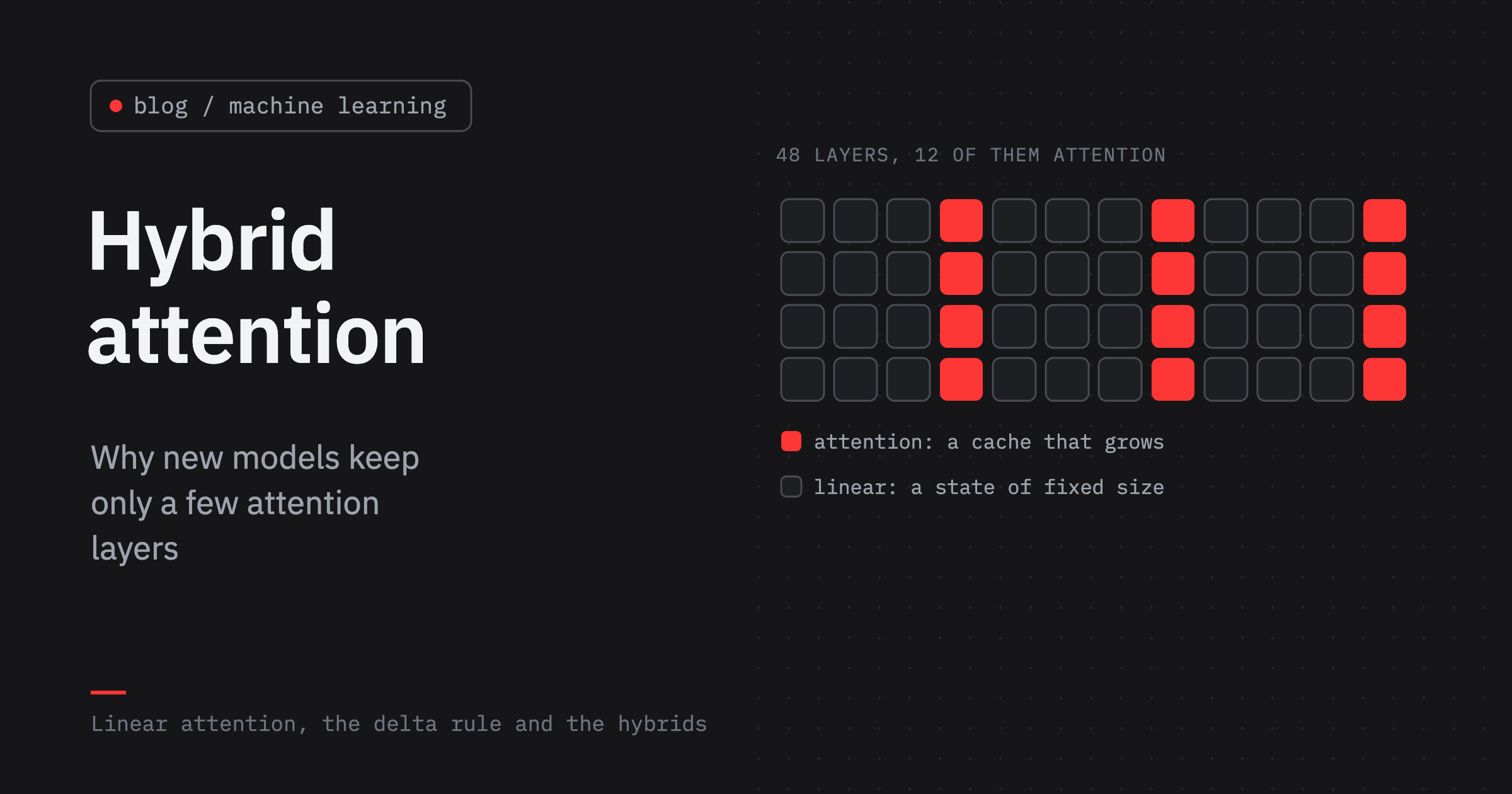
Qwen3-32B, a dense model from April 2025, keeps 32 GiB of keys and values for one conversation of 128 thousand tokens, about half of what its weights take. Qwen3-Next, released by the same team a few months later, keeps 3 GiB at the same length. It doesn’t compress its cache or skip tokens.

Three of every four of its layers simply have no cache: they read the text the way a recurrent network does, into a state of fixed size, and only every fourth layer is ordinary attention.

Qwen3-Next is not the only one. Jamba, the Nemotron-H models, Kimi Linear and, for a while, MiniMax made the same choice: full attention in a few layers, something cheaper in the rest.

This post builds the cheaper part from scratch, from linear attention to the gated delta rule, tests what it can and cannot remember, and then looks at how real models combine the two and what that buys on a GPU.

What attention remembers

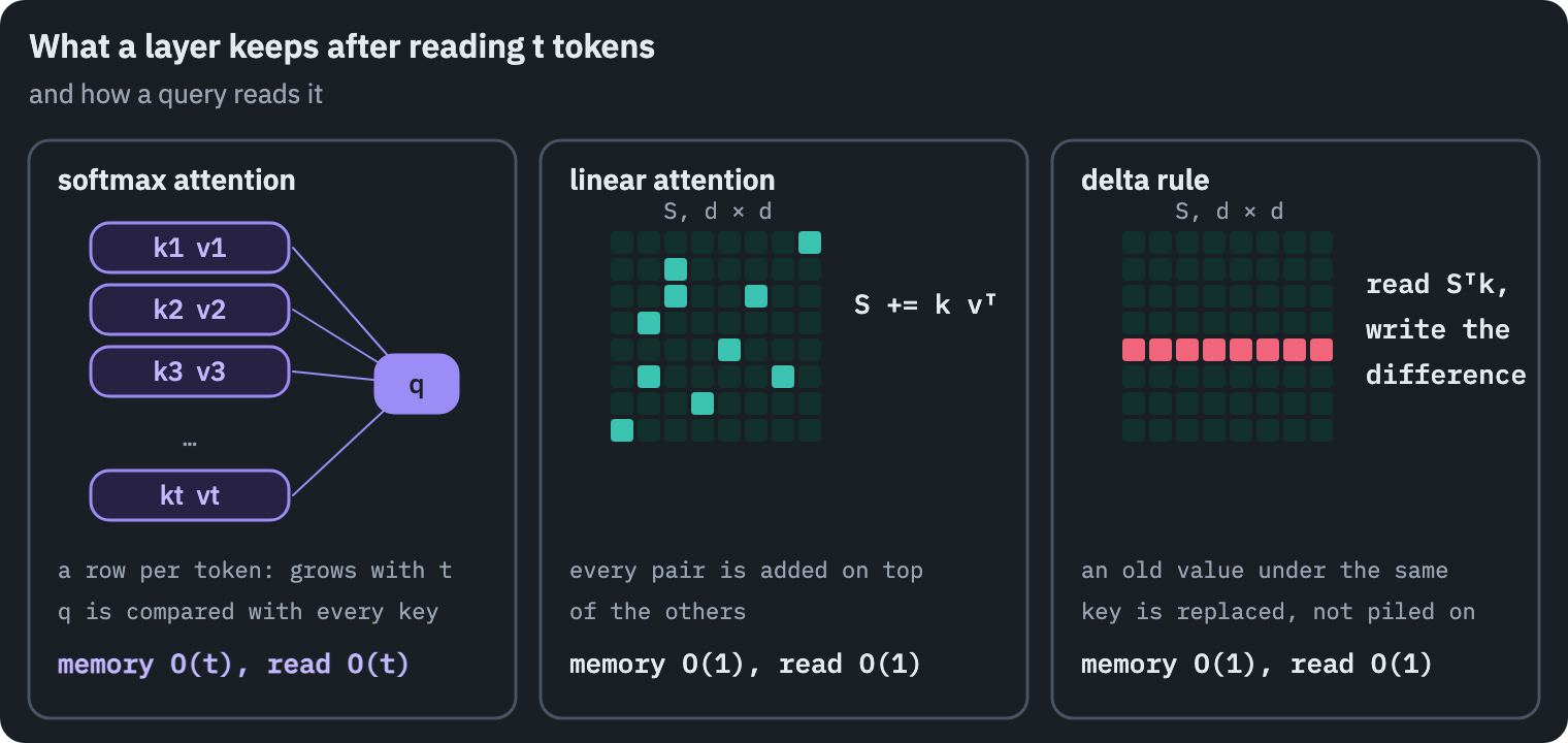
Every attention layer of a Transformer answers the same question for every token: which of the earlier tokens matter here, and what do they say. Softmax attention answers it by brute force. Each token leaves behind a key, which says what it is about, and a value, which says what it contributes.

A new token arrives with a query, compares it with every key, turns the scores into weights with a softmax, and takes the weighted sum of the values:

Nothing is ever thrown away. To write token \(t\), the layer needs the keys and values of all \(t-1\) tokens before it, which is why serving engines keep them in a KV cache instead of recomputing them.

Memory therefore grows linearly with the text, and since each new token reads all of it, reading a whole text of \(n\) tokens takes time proportional to \(n^2\).

Think of a library that keeps every book it has ever received and checks the whole catalogue for every question. The answers are exact, but the building has to grow with the collection.

Attention without the softmax

The softmax is what forces the rereading: the exponential ties every query to every key. Katharopoulos and colleagues replaced it, putting a dot product of features \(\phi(q) \cdot \phi(k)\) in place of \(\exp(q \cdot k)\), with a positive map such as \(\phi(x) = \mathrm{elu}(x) + 1\), and noticed that the rest follows from associativity^[1]:

The query no longer sits inside the sum. Everything the layer needs from the past now sits in \(S_t\), a \(d \times d\) matrix, and \(z_t\), a vector, and both are updated by adding one term per token:

This is a recurrent network. Its state has the same size after ten tokens and after ten million, writing a token costs the same at any position, and there is no cache. Done for all positions at once, the same computation is the attention formula with the brackets moved:

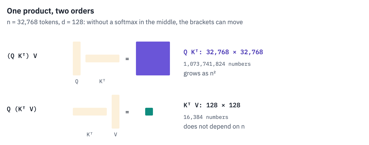
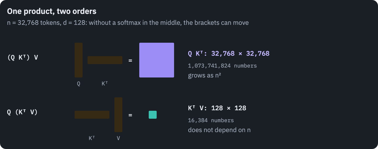
Both forms compute the same numbers, only in a different order. In code, the recurrent form loops over positions and the parallel one builds the masked score matrix:

def linear_recurrent(q, k, v):
    q, k = feature(q), feature(k)
    state = q.new_zeros(*q.shape[:2], q.shape[-1], v.shape[-1])  # S = sum of k v^T
    norm = q.new_zeros(*q.shape[:2], q.shape[-1])                # z = sum of k
    out = []
    for t in range(q.shape[2]):
        state = state + k[:, :, t, :, None] * v[:, :, t, None, :]
        norm = norm + k[:, :, t]
        out.append(torch.einsum("bhk,bhkv->bhv", q[:, :, t], state)
                   / torch.einsum("bhk,bhk->bh", q[:, :, t], norm)[..., None])
    return torch.stack(out, dim=2)

def linear_attention(q, k, v):
    q, k = feature(q), feature(k)
    causal = torch.ones(q.shape[2], q.shape[2], dtype=torch.bool).tril()
    scores = (q @ k.transpose(-1, -2)).masked_fill(~causal, 0)
    return (scores @ v) / scores.sum(-1, keepdim=True)

On random inputs in double precision the two functions agree to about \(10^{-15}\), which is rounding error. The recurrent form is how the layer writes text, one token at a time; the parallel form is how it trains, all positions at once.

The parallel form also shows a catch: it still builds an \(n \times n\) matrix of scores, because with a causal mask every position needs its own prefix of the sum and the brackets can’t simply move. Training a linear layer efficiently needs a third form, which comes later.

A memory of fixed size

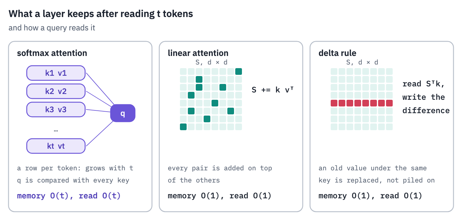
The price of the fixed state can be read straight from the formula. The state is one matrix. Every pair \((k_j, v_j)\) is added into the same \(d^2\) numbers, and to recall the value stored under a key, the layer multiplies the state by it:

The first term is the stored value. The second is interference: every other pair, weighted by how similar its key is to \(k_i\). If the keys are orthogonal, the interference is exactly zero, but a \(d\)-dimensional space has room for only \(d\) orthogonal directions.

Beyond that, each new pair blurs the ones already stored. The library has turned into one notebook page on which every note is written over the others; it stays readable while there are few notes.

Softmax attention has no such limit because it never mixes the notes: it keeps them all and lets the exponential pick out the right one. It pays for that with the growing cache. Everything below is about this trade between a fixed state and exact recall.

Arora and colleagues measured it across efficient architectures and called it “a key tradeoff between a model’s state size and recall ability”^[2]: the smaller the state a model keeps while reading, the worse it recalls.

Writing with the delta rule

Plain addition has a second, quieter problem. If the same key comes back with a new value, say a variable that has been reassigned, the state holds the sum of the old and the new value, and reading it returns a mixture of both. Nothing in the notebook can be crossed out.

The remedy dates from 1960, when Widrow and Hoff trained their linear neurons with what became known as the delta rule: compare the output with the target and move the weights in proportion to the error^[3].

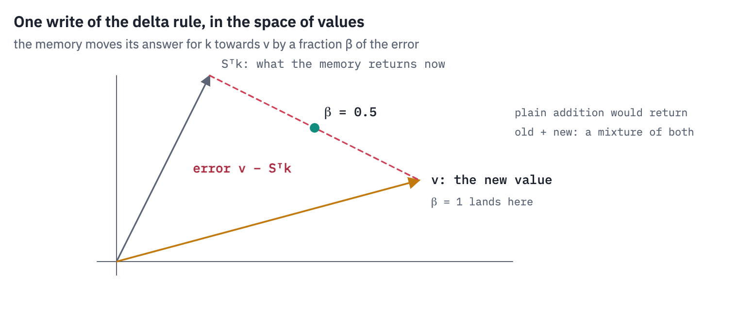
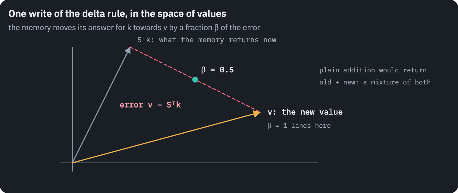
Schlag, Irie and Schmidhuber noticed that the state of linear attention is a weight matrix, written at every step, and proposed writing it the same way^[4]. Before storing \(v_t\) under \(k_t\), read what is already there, and write only the difference:

with \(k_t\) of unit length and \(\beta_t \in (0, 1)\), a writing strength the layer computes for each token. This is one step of gradient descent on the memory’s error for this key, \(\tfrac12 \lVert S^\top k_t - v_t \rVert^2\), with learning rate \(\beta_t\): the gradient with respect to \(S\) is \(k_t (S^\top k_t - v_t)^\top\).

With \(\beta_t = 1\), the old value under \(k_t\) is erased and the new one is stored exactly. A layer that writes this way is called DeltaNet. In the space of values, one write looks like this:

Side by side, the three memories differ in what they keep and in how a new pair changes it:

How much of a difference does editing make? A small experiment shows both sides of it: a \(64 \times 64\) memory, random unit keys and values, written once by adding and once by the delta rule, and read back by finding the nearest stored value. Softmax attention, which keeps every pair, is the reference.

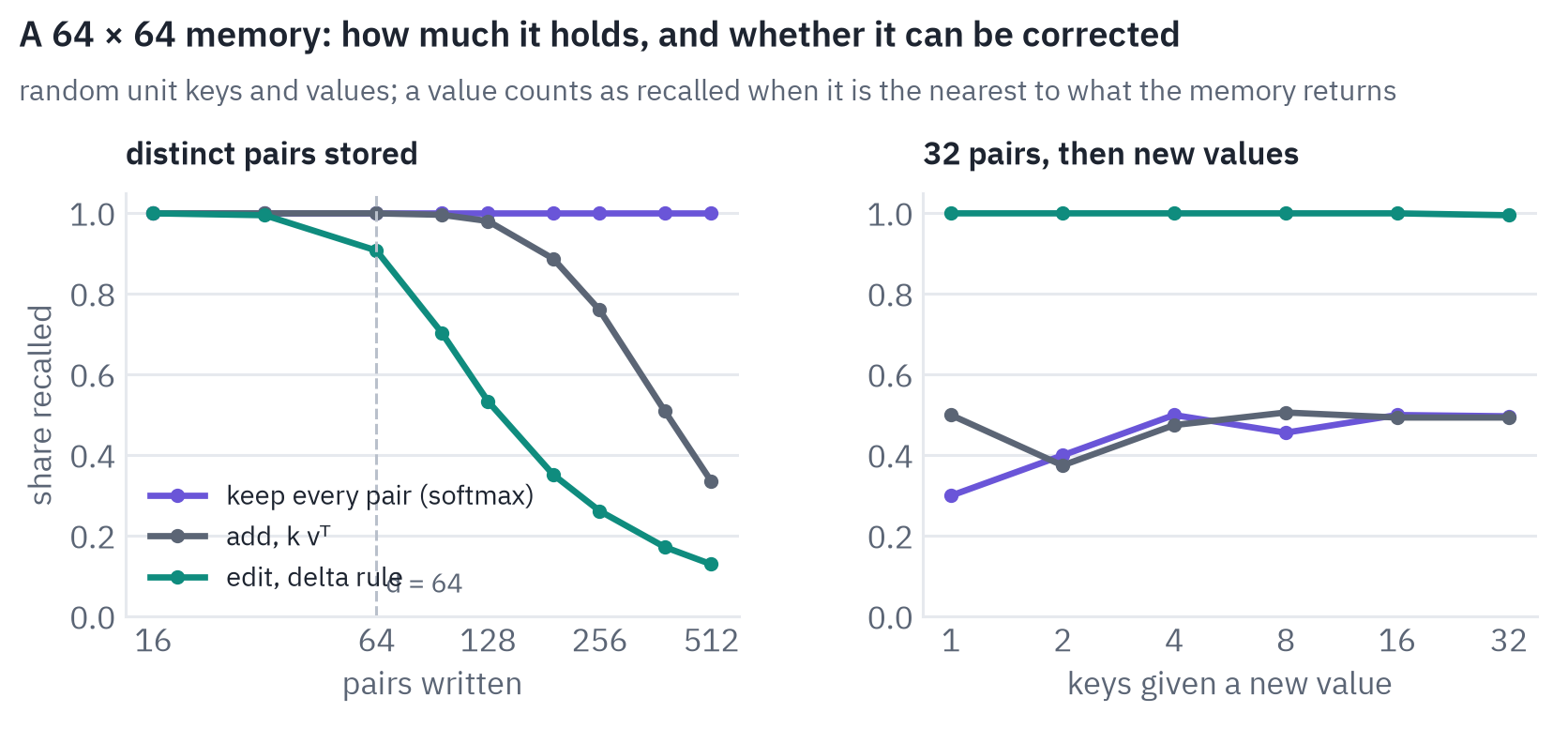
The left panel holds a surprise: from 64 pairs on, plain addition recalls more than the delta rule. With \(\beta_t = 1\), each write makes the memory return exactly \(v_t\) for \(k_t\), and since random keys are not orthogonal, it also shifts what the memory returns for every older key that overlaps with \(k_t\).

Once the memory is full, the delta rule holds the recent pairs well and the old ones poorly. Addition keeps a blur of everything, in which the nearest value is still often the right one.

The right panel shows what the delta rule is for. After 32 pairs, some of the keys get a new value. The delta rule returns the new value nearly every time.

Addition returns the sum of the old and the new value, which is nearer to the new one only about half the time, and softmax attention as written here does no better: it sees two identical keys and averages their values.

A trained Transformer can tell the later pair from the earlier one by their positions; this toy has no positions.

So the delta rule doesn’t enlarge the memory. A \(d \times d\) matrix stays a \(d \times d\) matrix, and it holds at most \(d\) pairs exactly, whichever way they are written. What the delta rule adds is the ability to correct what is stored, which plain addition doesn’t have at all.

Forgetting on purpose

Editing handles values that change. It does nothing about the opposite problem: a long text moves on, and much of what the state holds stops mattering. A memory of fixed size needs a way to let go of it.

That is what gates are for. RetNet multiplied the state by a fixed decay at every step^[5], Gated Linear Attention made the decay depend on the token^[6], and Mamba-2 showed that its own selective state space model is linear attention with a data-dependent scalar gate^[7]. Gated DeltaNet puts the gate and the delta rule together^[8]:

Both \(\alpha_t\) and \(\beta_t\) are computed from the current token, so the layer decides as it reads when to forget and how firmly to write.

The two parts split the work: in the authors’ words, the gate “can promptly clear memory by setting \(\alpha_t \to 0\)”, and with \(\alpha_t \to 1\) the layer is “effectively switching to the pure delta rule” and edits single entries without touching the rest.

This is the layer Qwen3-Next is built on, and Kimi Delta Attention is the same update with a separate gate for every channel of the state instead of one per head^[9].

Training a recurrence in parallel

A recurrence over positions is awkward to train on a GPU, which is fast at large matrix products and slow at loops of ten thousand small updates. The solution is to cut the sequence into chunks.

Inside a chunk of 64 tokens, the writes depend on each other only through a small lower-triangular system that can be solved with matrix products; between chunks, only the \(d \times d\) state is passed along^[10].

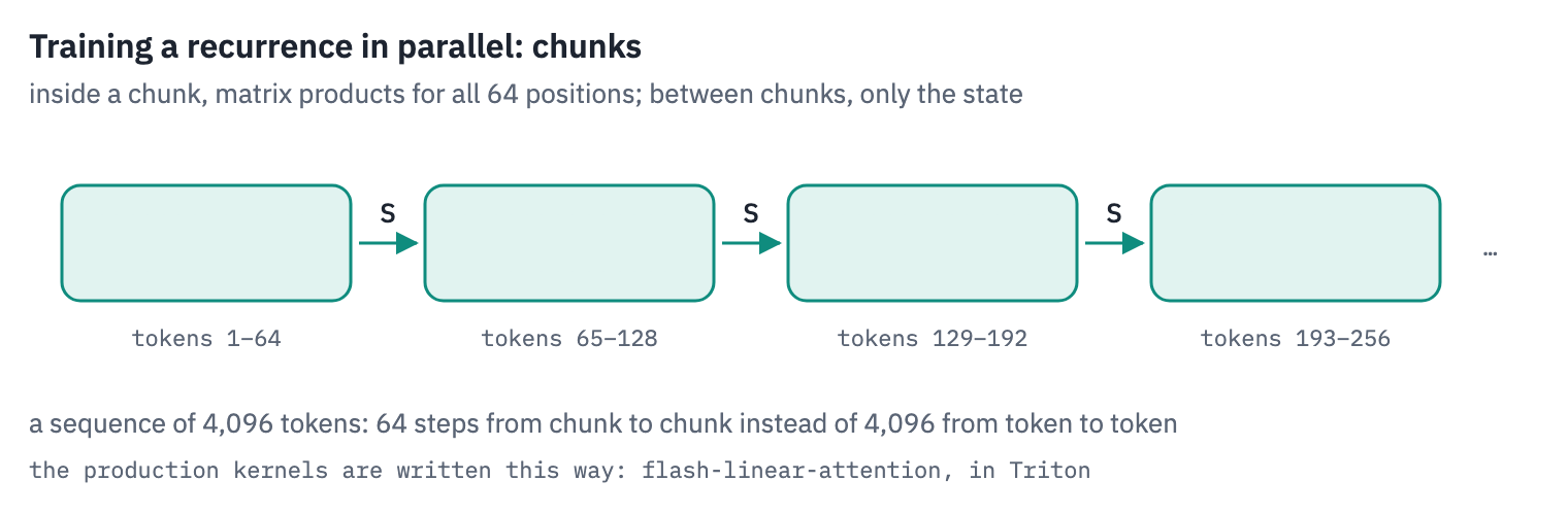
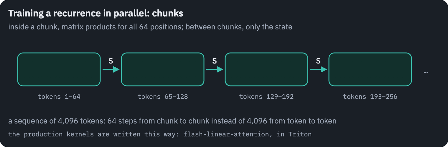
The chunked form is exact. My plain-PyTorch version of it agrees with the token-by-token loop to \(1.4 \times 10^{-15}\) in double precision, with the gate or without it, and it is what the experiments below train with. Production models use the Triton kernels of flash-linear-attention, which do the same thing much faster.

A test of memory: associative recall

The language modelling loss says little about memory, because much of predicting the next word needs little of it. A more direct test asks a model to remember what it was told. In multi-query associative recall, a sequence lists key-value pairs and then asks for the values of the keys in a shuffled order^[11]:

k1 v1  k2 v2  ...  kN vN   |   q1 a1  q2 a2  ...  qN aN

Each \(q_i\) is one of the keys, and the model must put the right value after it. It is the skill behind answering a question about a long document, using a name defined forty pages earlier, or calling a function with the arguments described at the top of a prompt.

I trained six small models on it, each with four layers of width 64 and two heads, the same in everything except how their layers mix tokens: softmax attention in all four, linear attention, DeltaNet, Gated DeltaNet, and two hybrids with three Gated DeltaNet layers and one softmax attention layer.

In one hybrid the attention layer is second; in the other it is on top, the place it has in each block of four in Qwen3-Next.

Every layer, attention included, first passes its queries, keys and values through a short convolution over the last four positions, as Mamba and DeltaNet do, so that a value can carry its key with it.

Each model saw 64 fresh random sequences at each of 4,000 steps and was scored on held-out ones. The models with Gated DeltaNet layers trained on an Apple M2, the others on a T4 (code).

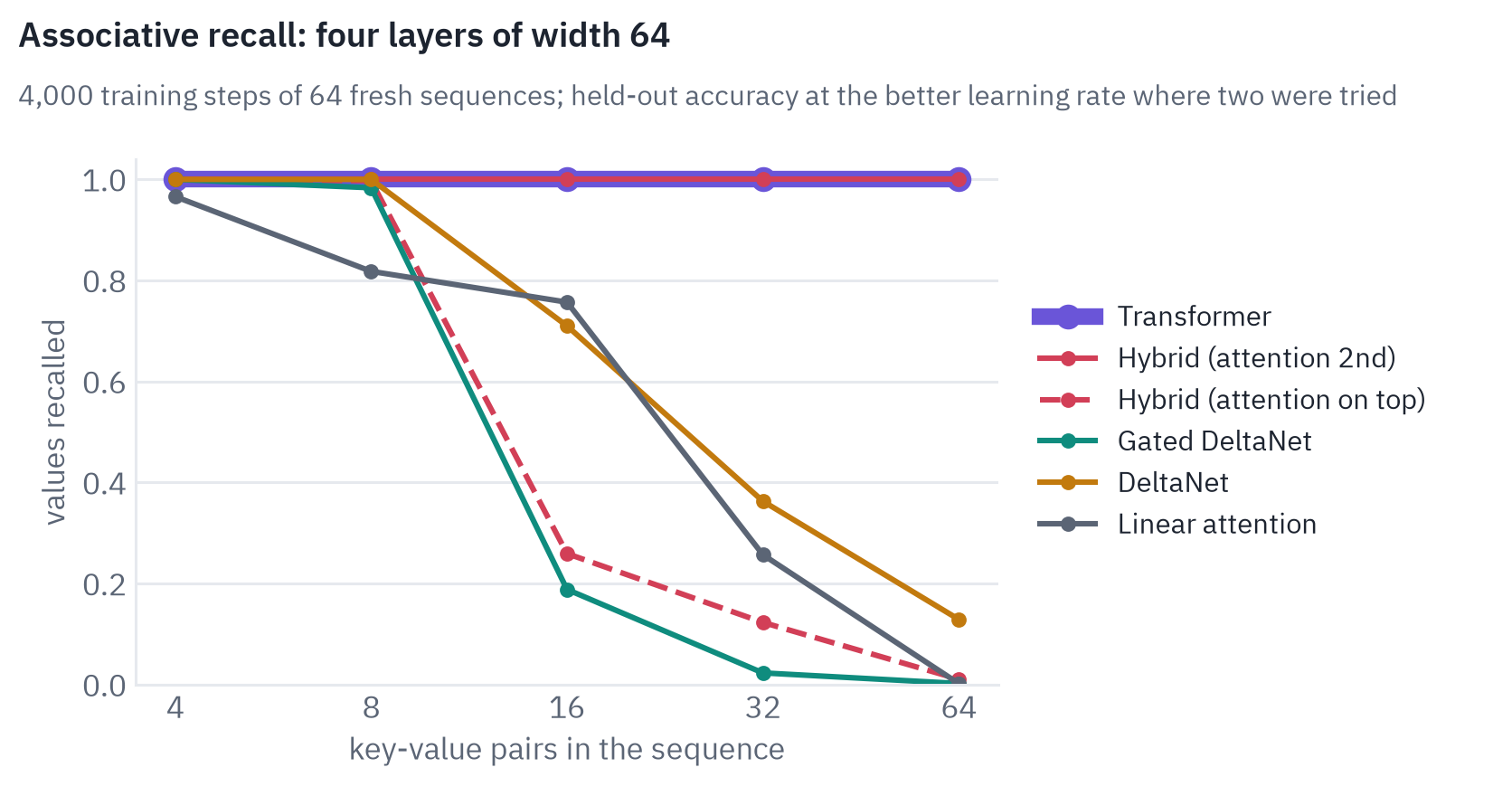
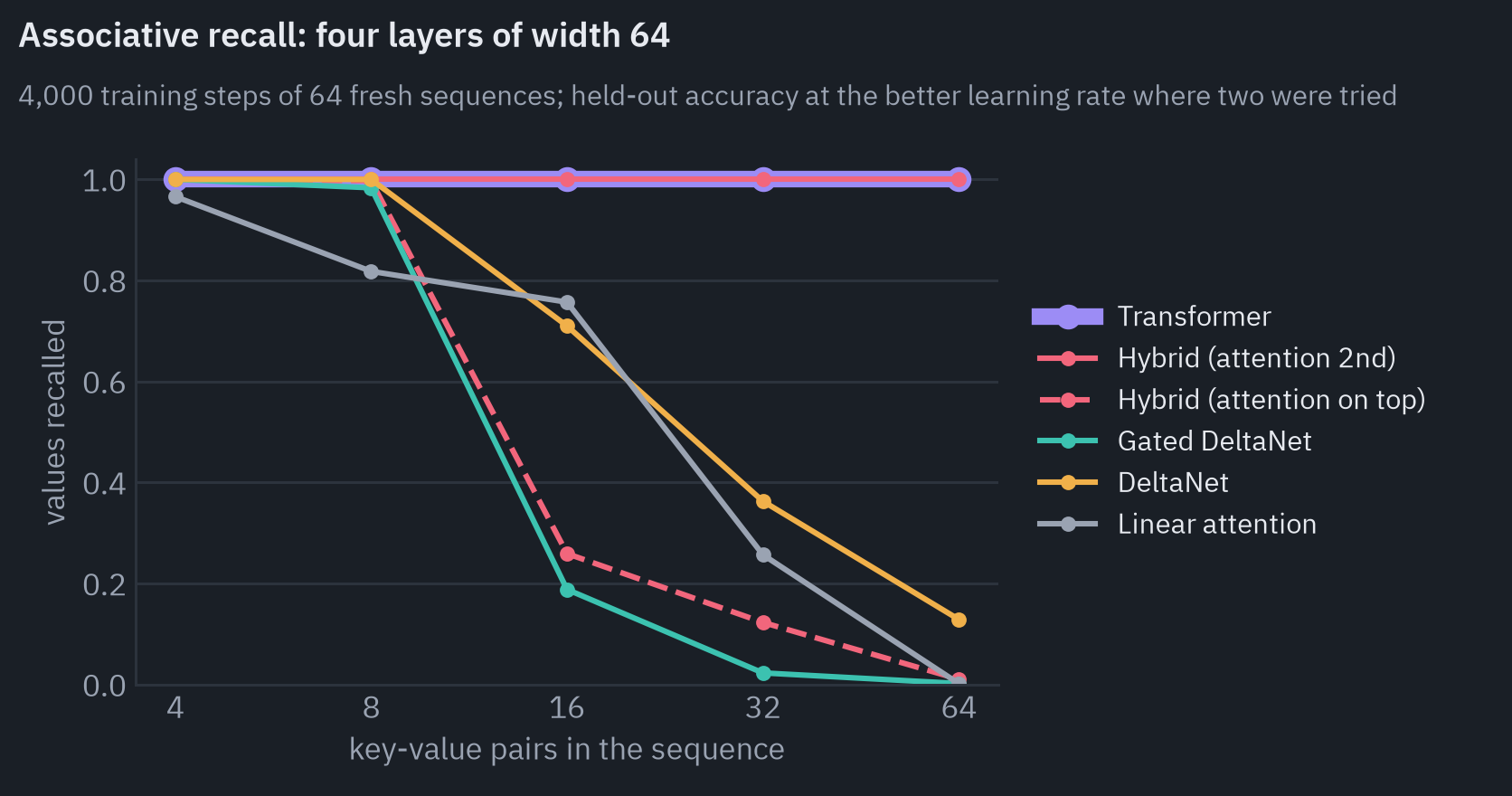
The Transformer recalls every value at every size on the chart. The three recurrent models hold up while there are few pairs and fall apart between 8 and 32: at 32 pairs DeltaNet recalls 36% of the values, linear attention 26% and Gated DeltaNet 2%, and at 64 the best of them, DeltaNet, recalls 13%.

Each head here works with keys of 32 numbers, so by the bound from earlier its state holds at most 32 pairs exactly, and at 16 pairs all three are already well short of full recall.

At 128 pairs even the Transformer didn’t learn the task in 4,000 steps, which is why the chart stops at 64.

Gated DeltaNet, the newest of the three, comes last from 16 pairs on. That is less strange than it looks, because this test gives the gate nothing to do. Every pair has to be kept until its question comes, so forgetting can only lose information.

The authors of Gated DeltaNet, who trained models of 1.3 billion parameters on 100 billion tokens of real text, found that it “consistently surpasses existing models like Mamba2 and DeltaNet”, in-context retrieval included^[8]. Four layers and 4,000 steps of a synthetic task are a different regime.

The gate is also the easiest part to get wrong. In my first version it started at about one half, and weight decay kept pulling it back there, so the state lost half of what it held at every token, and Gated DeltaNet and the hybrid stayed at chance level.

Starting the gate as the Gated DeltaNet and Mamba-2 code does, where a typical head keeps about 94% of its state from one token to the next, and leaving it out of weight decay, fixed it.

The two hybrids differ only in the order of their layers. With attention second, the hybrid recalls every value at every size, like the Transformer, though three of its four layers are Gated DeltaNet, which on its own recalls the least.

With attention on top, the same layers recall 26% of the values at 16 pairs and 12% at 32, at the better of two learning rates: a little more than Gated DeltaNet alone and less than DeltaNet.

I can’t say for certain why. The attention layer on top has what it needs: the convolution hands each value its key, and the other hybrid shows that one attention layer among three Gated DeltaNet layers is enough. This one just doesn’t learn the lookup in 4,000 steps.

A model of four layers is far from Qwen3-Next, where twelve attention layers are spread through 48 and most of them have many recurrent layers on both sides, so this says nothing about whether its layout is a good one.

It does show that the ratio alone doesn’t describe a hybrid. With the same layers in a different order, one model recalled like a Transformer and the other like a recurrent network.

Why one layer of attention is enough

Attention solves associative recall in one layer: the query for \(k_i\) meets the stored key \(k_i\), the softmax puts nearly all the weight on it, and out comes \(v_i\), however many pairs came before.

Arora and colleagues proved that attention needs a model dimension independent of the sequence length for this, while the gated convolutions they studied need one that grows with it.

Measuring the gap in quality between the two kinds of models on real text, they found that “82% of the gap is explained by each model’s ability to recall information that is previously mentioned in-context”^[11].

Copying gives the same picture. Jelassi and colleagues proved that two layers of attention can copy strings of exponential length, while models with a fixed state are “fundamentally limited by their fixed-size latent state”^[12].

None of this requires attention everywhere. Much of predicting the next token is local, or a matter of keeping a running summary of what the text is about, and a gated recurrent layer does that well and cheaply.

Exact lookups into the distant past are rarer, and a layer that can make them serves the whole model: the recurrent layers around it carry the local context, the attention layer finds the match. In the library picture, most floors work from a notebook page, and every few floors someone is allowed into the archive.

The authors of Mamba-2 tried such hybrids and described the division of labour the same way: “attention layers act as a retrieval mechanism to quickly refer to previous tokens in the sequence instead of forcing the model to compress all the context to its memory”. They found that “around 10% of the total number of layers being attention performs best”^[7].

A study at NVIDIA trained an 8-billion-parameter Transformer, pure Mamba and Mamba-2 models and a hybrid with 4 attention layers out of 56 on the same data.

The pure Mamba models began to fail at looking up a number in a phone book beyond about 500 tokens. The hybrid exceeded the Transformer on all 12 standard tasks the authors evaluated, by 2.65 points on average^[13].

Hybrids in practice

The first large hybrid was Jamba from AI21, in March 2024: Mamba layers with one attention layer in every eight^[14]. MiniMax, NVIDIA, Qwen and Moonshot followed, each with its own recurrent layer and its own ratio.

MiniMax-Text-01 put one softmax layer after every seven layers of lightning attention, a fast form of linear attention, after finding that lightning attention alone “demonstrates limited retrieval capabilities”^[15]. NVIDIA’s Nemotron-H models keep “roughly 8% of the total number of layers” as attention, and the rest are Mamba-2 and MLP layers^[16].

Qwen3-Next uses Gated DeltaNet in three layers out of four. According to the Qwen team, at this ratio “the model consistently outperforms any monolithic architecture”^[17].

Kimi Linear uses Kimi Delta Attention, the variant with a gate for every channel, also at 3:1. It leaves word order entirely to the recurrent layers: its attention layers use no positional encoding at all^[9].

Here is where each model keeps its full attention, read from the config files the models are published with:

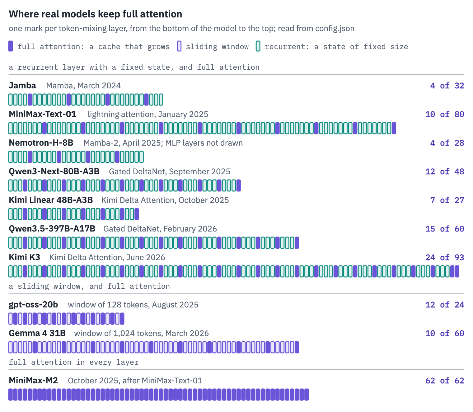
Drawn to scale, the designs differ more than their headline ratios. Jamba and MiniMax-Text-01 keep one attention layer in eight, Nemotron-H-8B 4 of its 28 token-mixing layers, the Qwen and Kimi models one in four.

Kimi Linear’s released model has 27 layers, so its 3:1 turns into 20 recurrent layers and 7 attention layers, the last one attention.

Kimi K3, 93 layers deep, adds an extra attention layer at the top, “ensuring that the final layer always performs global attention”^[18]. All of them spread the attention layers evenly through the depth.

The second group shrinks the cache in another way. gpt-oss and Gemma use softmax attention in every layer, but most of their layers see only a sliding window of recent tokens: 128 in gpt-oss, where windowed and full layers alternate^[19], and 1,024 in Gemma 3, with five windowed layers for every full one^[20].

Gemma 4 kept the ratio. A window is the opposite trade to a recurrent state: it keeps recent tokens exactly and forgets older ones completely, while a state keeps a blurred summary of everything.

The last row is MiniMax-M2, the successor of MiniMax-Text-01, with full attention in all 62 layers. The team explained why in a blog post.

Small hybrids had matched full attention on the leaderboards, but “the price paid became obvious at a larger scale: the model had clear deficits in complex, multi-hop reasoning tasks”^[21].

The Qwen and Kimi hybrids keep more attention than MiniMax-Text-01 did, one layer in four rather than one in eight, and use the delta rule, which lightning attention lacks. Still, the episode is a fair warning that parity on small models and leaderboards doesn’t settle the question.

What the hybrids save is easiest to see in memory. For each model, the size of its cache follows from the config: the number of attention layers, key-value heads and head dimension.

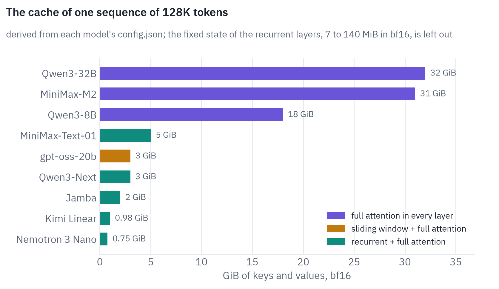
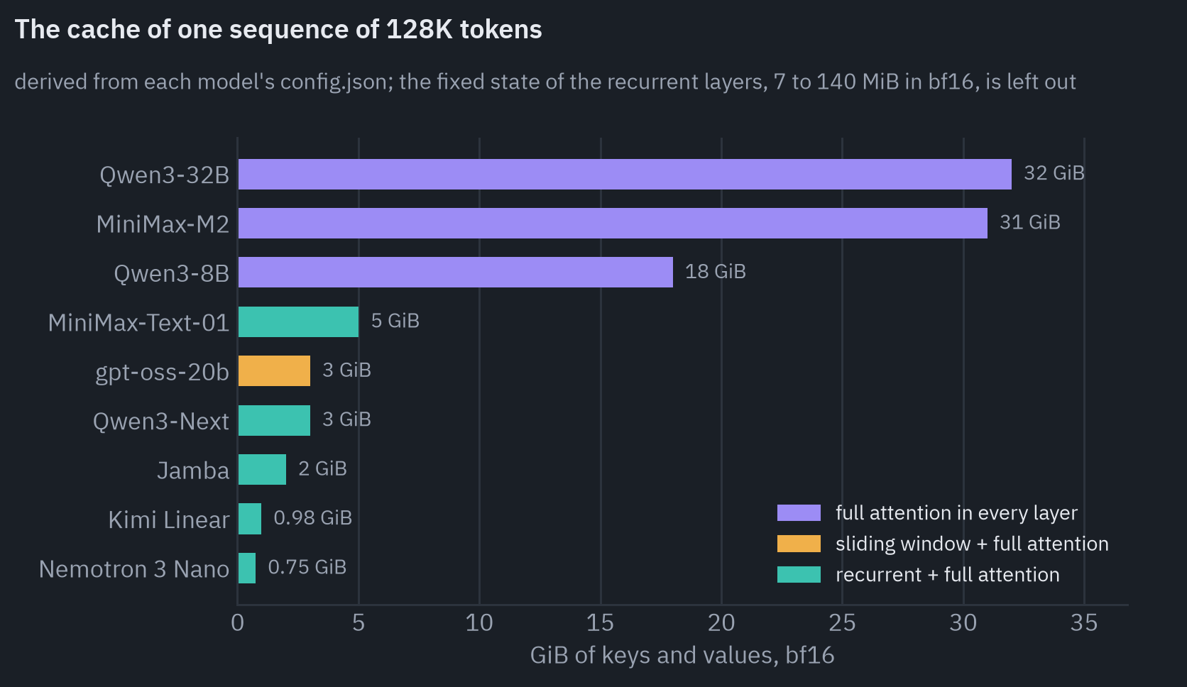
For one sequence of 128K tokens, Qwen3-Next keeps 3 GiB of keys and values, against 32 GiB for Qwen3-32B. Not all of the factor of ten comes from the hybrid. Each attention layer of Qwen3-Next keeps two key-value heads of 256 dimensions, where Qwen3-32B keeps eight of 128, which halves the cache per layer.

The rest, a factor of 5.3, is 12 attention layers instead of 64. The recurrent layers add a state of 36 MiB that stays the same at any length.

Kimi Linear starts from multi-head latent attention, introduced in DeepSeek-V2^[22], which already caches one compressed vector of 576 numbers per token and layer in place of keys and values for every head, and keeps it in 7 layers of 27.

That is 26% of the cache of an all-MLA model of the same depth, in line with the paper’s “reducing KV cache usage by up to 75%”. MiniMax-M2, at 31 GiB, keeps six times more than its predecessor.

At long context, the cache rather than the weights decides how many conversations fit on a GPU at once, and decoding speed follows from that.

The Kimi Linear authors measured decoding with a million tokens of context and put the result down to memory: the smaller cache “enables larger batches, yielding a 6.3× faster TPOT (1.84ms vs. 11.48ms) than MLA at 1M tokens”, TPOT being the time per output token.

What it costs on a GPU

The recurrent layer pays off only where the cache grows large, and a single layer on one GPU shows where that starts.

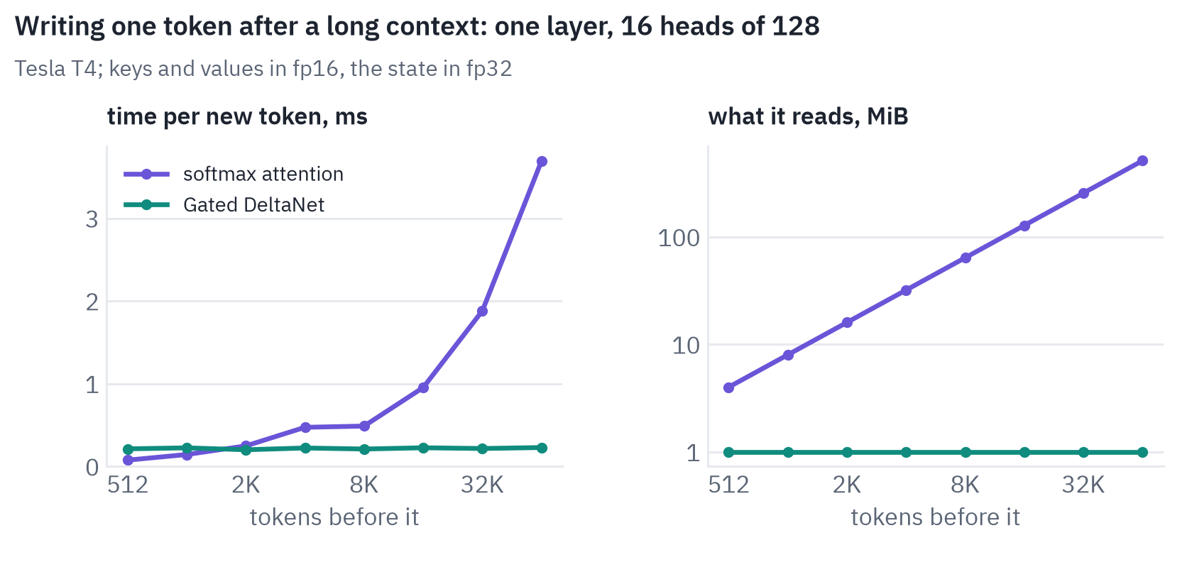
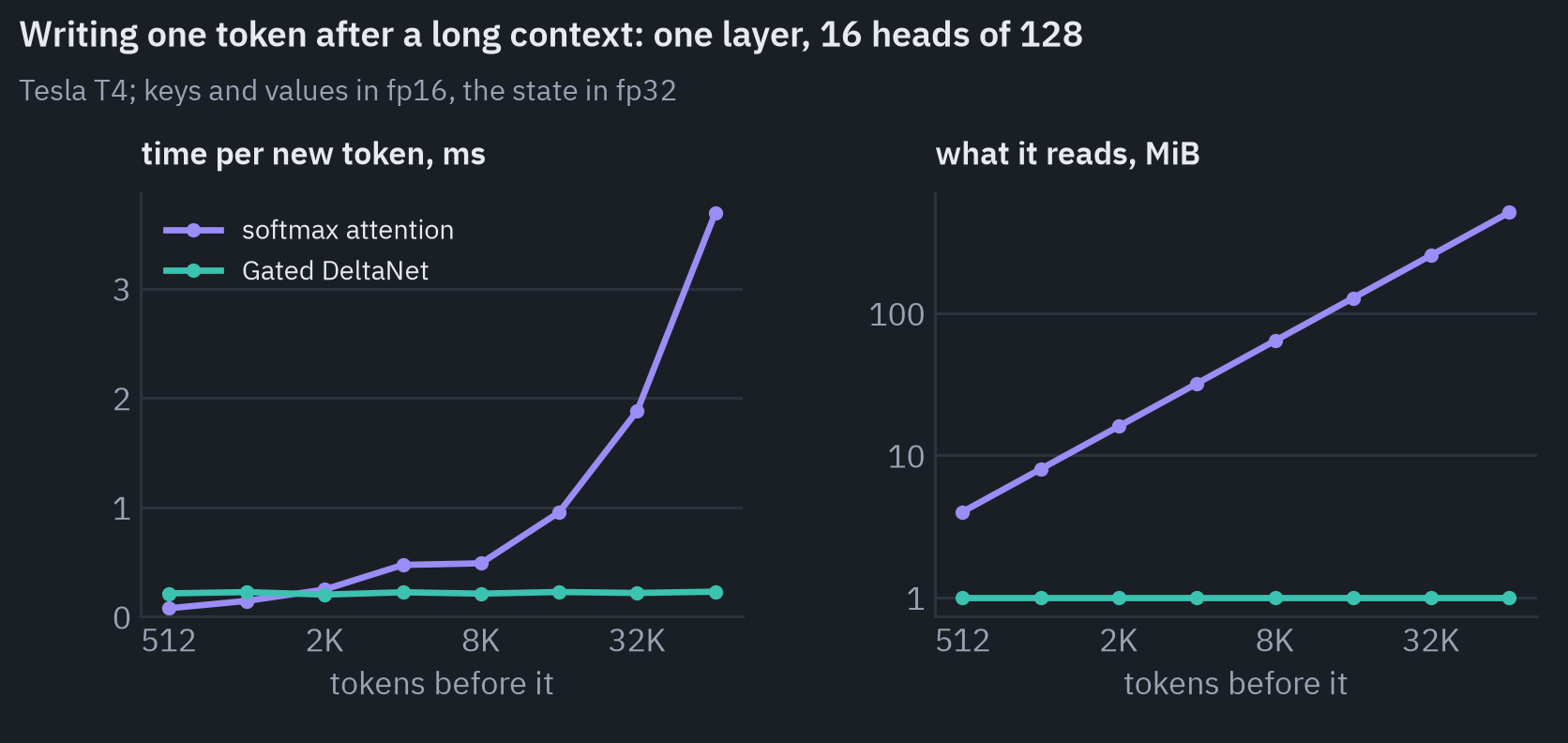
I timed one layer with 16 heads of 128 dimensions, about the size of a Gated DeltaNet layer in Qwen3-Next, in two situations: reading a prompt of \(n\) tokens at once, and writing one new token after \(n\) tokens.

Softmax attention runs through PyTorch’s fused attention kernel in half precision. Gated DeltaNet runs my plain-PyTorch chunked version in single precision, a Python loop over chunks of 64. The comparison is tilted against the recurrent layer on purpose: if it wins anyway, it wins on arithmetic, not on engineering.

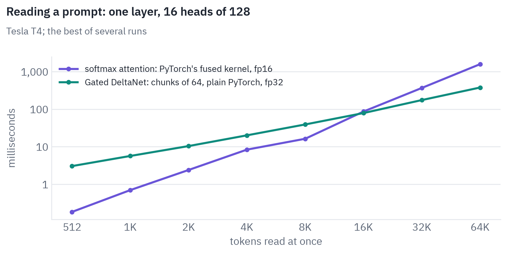
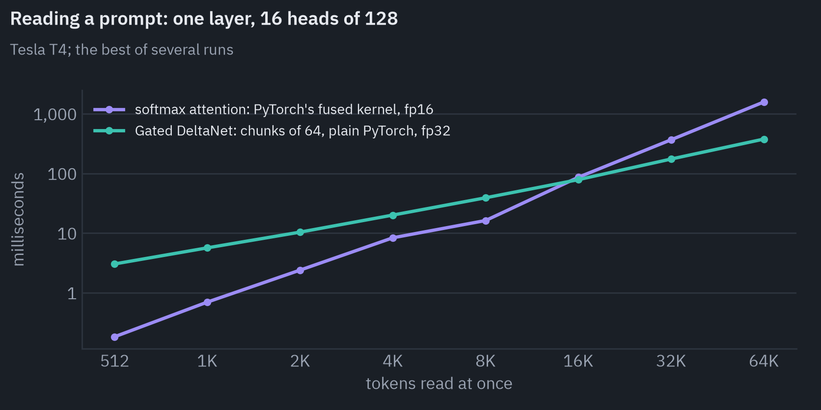
Reading a prompt, softmax attention is faster up to 8K tokens, which is no surprise: its kernel is one fused program, and mine is a loop. The slopes differ, though.

From 512 to 65,536 tokens, a sequence 128 times longer, the attention layer gets 8,600 times slower and the recurrent one 124 times slower. The curves cross between 8K and 16K tokens, and at 65K the recurrent layer is 4.2 times faster.

Writing a token is where the cache costs most. Attention reads the keys and values of every earlier token, 512 MiB at 65K tokens in this one layer, and its time grows in proportion, from 0.08 ms to 3.7 ms. The recurrent layer updates a state of 1 MiB and takes 0.2 ms at any length; at that size the time is mostly the overhead of launching a few small GPU kernels.

From about 2K tokens on, the recurrent step is faster, and at 65K it is 16 times faster.

One layer and one sequence understate the difference in a real server. There, the caches of all the conversations in a batch have to fit in memory at once, so a model whose cache is a quarter or an eighth of the size can serve proportionally more conversations at the same length.

Kimi Linear’s 6.3 times, quoted above, comes from exactly that. The attention layers of a hybrid still pay the full price; three quarters of its layers stop paying it.

When a hybrid is the right choice

A hybrid pays off when contexts are long and there are many of them: agents that carry long transcripts of tool calls, reasoning models that write tens of thousands of tokens, questions over long documents, a server holding hundreds of such conversations at once.

There the cache is most of the memory and reading it is most of the decoding time, and cutting it by a factor of four to ten changes how many users one GPU can serve.

At short contexts the gain is smaller than the headlines suggest. According to Qwen, the decoding throughput of Qwen3-Next is nearly 4 times that of Qwen3-32B at 4K tokens and over 10 times beyond 32K^[17].

But Qwen3-Next activates 3 billion parameters per token and Qwen3-32B all 32 billion, so the comparison mixes two savings, the mixture of experts and the hybrid, and the blog doesn’t separate them. The hybrid’s share is the part that grows with the context.

The costs are of three kinds. The first is quality on the tasks attention is best at, precise retrieval and multi-hop reasoning over long inputs: the deficits that sent MiniMax back to full attention.

The second is engineering. Recurrent layers need their own kernels, and serving tricks built around a cache of separate tokens get harder when part of the model keeps a state that has absorbed all of them.

Reusing the cache of a shared prompt needs copies of the state saved at chosen positions, and rolling back a rejected speculative token needs the state from a step earlier.

The third is that the field keeps moving. Qwen3.8-Flash-Next replaced the full attention layers of its hybrid with sparse attention^[23], and DeepSeek-V4 combines two kinds of compressed attention instead of adding recurrent layers^[24]. Both directions go after the same cache.

A hybrid’s way is to give most layers a memory of fixed size and to keep a few that can still read every token.

References

1. Katharopoulos, A., Vyas, A., Pappas, N., & Fleuret, F. (2020). Transformers are RNNs: fast autoregressive Transformers with linear attention. ICML 2020. ↩
2. Arora, S., et al. (2024). Simple linear attention language models balance the recall-throughput tradeoff. ICML 2024. ↩
3. Widrow, B., & Hoff, M. E. (1960). Adaptive switching circuits. IRE WESCON Convention Record, 4, 96–104. ↩
4. Schlag, I., Irie, K., & Schmidhuber, J. (2021). Linear Transformers are secretly fast weight programmers. ICML 2021. ↩
5. Sun, Y., et al. (2023). Retentive network: a successor to Transformer for large language models. arXiv. ↩
6. Yang, S., Wang, B., Shen, Y., Panda, R., & Kim, Y. (2024). Gated linear attention Transformers with hardware-efficient training. ICML 2024. ↩
7. Dao, T., & Gu, A. (2024). Transformers are SSMs: generalized models and efficient algorithms through structured state space duality. ICML 2024. ↩
8. Yang, S., Kautz, J., & Hatamizadeh, A. (2025). Gated delta networks: improving Mamba2 with delta rule. ICLR 2025. ↩
9. Kimi Team (2025). Kimi Linear: an expressive, efficient attention architecture. arXiv. ↩
10. Yang, S., Wang, B., Zhang, Y., Shen, Y., & Kim, Y. (2024). Parallelizing linear Transformers with the delta rule over sequence length. NeurIPS 2024. ↩
11. Arora, S., et al. (2023). Zoology: measuring and improving recall in efficient language models. ICLR 2024. ↩
12. Jelassi, S., Brandfonbrener, D., Kakade, S. M., & Malach, E. (2024). Repeat after me: Transformers are better than state space models at copying. ICML 2024. ↩
13. Waleffe, R., et al. (2024). An empirical study of Mamba-based language models. arXiv. ↩
14. Lieber, O., et al. (2024). Jamba: a hybrid Transformer-Mamba language model. arXiv. ↩
15. MiniMax (2025). MiniMax-01: scaling foundation models with lightning attention. arXiv. ↩
16. NVIDIA (2025). Nemotron-H: a family of accurate and efficient hybrid Mamba-Transformer models. arXiv. ↩
17. Qwen Team (2025). Qwen3-Next: towards ultimate training & inference efficiency. Alibaba Cloud blog. ↩
18. Kimi Team (2026). Kimi K3: open frontier intelligence. arXiv. ↩
19. OpenAI (2025). gpt-oss-120b & gpt-oss-20b model card. arXiv. ↩
20. Gemma Team (2025). Gemma 3 technical report. arXiv. ↩
21. MiniMax (2025). Why did MiniMax M2 end up as a full attention model? Hugging Face blog. ↩
22. DeepSeek-AI (2024). DeepSeek-V2: a strong, economical, and efficient mixture-of-experts language model. arXiv. ↩
23. Qwen Team (2026). Qwen3.8-Flash-Next model card. Hugging Face. ↩
24. DeepSeek-AI (2026). DeepSeek-V4: towards highly efficient million-token context intelligence. arXiv. ↩