Contents
Transformer architectures: from BERT to diffusion · lesson 3 of 15 · all lessons · run on Kaggle · open in Colab · code on GitHub
In 2019 BERT was the best reader of English and one of the worst search engines. Ask it which two of 10,000 sentences mean the most similar things, and it has to read every pair, which “requires about 50 million inference computations (~65 hours)”.
Nils Reimers and Iryna Gurevych at TU Darmstadt changed one thing: they made BERT write down what it read as one vector per sentence, so that comparing two texts became a dot product. The same search then took “about 5 seconds”[1].
Their Sentence-BERT now sits, under various names, behind most of the search you meet: the retrieval half of every RAG system, “related articles”, duplicate detection, the search box of a documentation site. It also has rivals with very different trade-offs, and a thirty-year-old formula that none of them can afford to ignore.
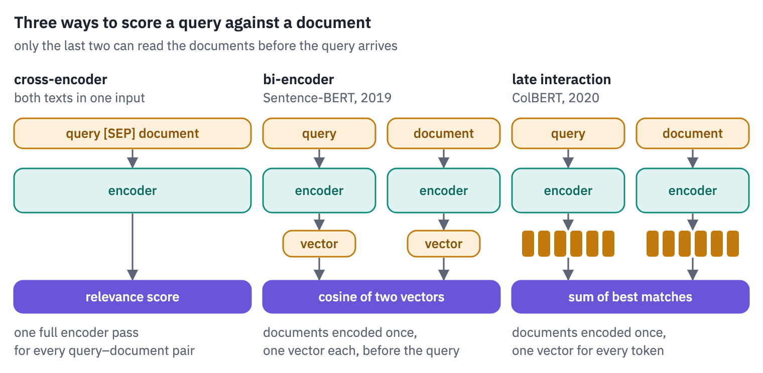
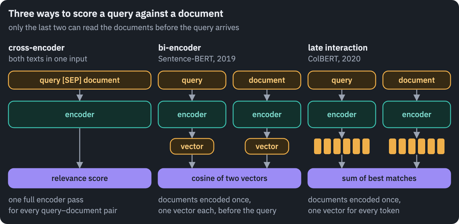
In this lesson you’ll build all three, check each against the real weights, and pit them against each other on a task where good search is easy to tell from bad: finding machine-learning papers from the questions researchers actually ask.
What you’ll do
- Write BM25, the formula every neural retriever still has to beat, and see how far counting words goes.
- See why an encoder’s own vectors are useless for search, and fix that the way Sentence-BERT does: train a bi-encoder with in-batch negatives, on nothing but the titles and abstracts of the papers themselves.
- Load the most downloaded model on the Hugging Face Hub into the same code, find out what a billion training pairs buy, and adapt it to the corpus in ten minutes.
- Write a cross-encoder reranker and ColBERT’s late interaction, and check both against the real weights.
- Assemble a search engine from the pieces, and measure what each costs in quality, time and memory.
What you need: a GPU. On Kaggle, Settings → Accelerator → GPU; on Colab, Runtime → Change runtime type → T4 GPU. The notebook downloads five small encoders and the titles and abstracts of 64,000 papers, and trains two encoders for ten minutes each; on a T4 it runs in about 45 minutes.
Setup
One small helper package, tfs, draws the course’s plots and token chips and knows where the notebook runs (Kaggle, Colab or your own machine). Everything the lesson teaches is written out in the notebook itself.
import importlib.util
import subprocess
import sys

TFS = "git+https://github.com/xmarva/transformers-from-scratch@main"
if importlib.util.find_spec("tfs") is None:
    subprocess.check_call([sys.executable, "-m", "pip", "install", "-q", TFS])

from tfs import env
from tfs.viz import table, token_chips, use_course_style

env.quiet()  # no progress bars or environment warnings in the outputs
SEED = 42
env.seed_everything(SEED)
COLORS = use_course_style()
WORK_DIR = env.work_dir()
import json
import math
import re
import string
import time
from collections import Counter, defaultdict

import matplotlib.pyplot as plt
import numpy as np
import pandas as pd
import torch
import torch.nn as nn
import torch.nn.functional as F
from huggingface_hub import hf_hub_download
from IPython.display import display
from safetensors.torch import load_file
from tfs.viz import bars, heatmap
from transformers import AutoTokenizer
# the reference implementations, for the checks
from transformers import AutoModelForSequenceClassification, BertModel

SMOKE = env.smoke()  # CI runs the lesson on a small slice; you run it in full
device = "cuda" if torch.cuda.is_available() else "cpu"
assert device == "cuda" or SMOKE, "This lesson encodes 58,000 papers six times: use a GPU."
if device == "cuda":
    print("GPU:", torch.cuda.get_device_name(0))
half = torch.float16 if device == "cuda" else torch.float32  # what indexes are stored in
GPU: Tesla T41. The task: 597 questions, 64,183 papers
LitSearch is a benchmark built at Princeton from the way researchers look for papers [2]. Some of its 597 questions were written by GPT-4 from paragraphs of real papers that cite other work, and ask for the paper behind the citation; the others were written by authors of ACL 2023 and ICLR 2024 papers about their own papers.
The benchmark’s authors checked every question by hand. The corpus is 64,183 papers from the ACL Anthology and ICLR, and each question names the one or few papers it is after.
The benchmark was not built to flatter anyone: in its paper, Google Search and research tools lagged behind the best neural retriever “by up to 32 recall points”.
The corpus files also hold the full text of every paper, more than a gigabyte of it. We need only titles and abstracts, and Parquet stores every column separately, so we read just those three columns straight from the Hugging Face Hub: about 35 MB instead of 1.2 GB.
LITSEARCH = "hf://datasets/princeton-nlp/LitSearch/"
queries = pd.read_parquet(LITSEARCH + "query/full-00000-of-00001.parquet")
shards = [pd.read_parquet(LITSEARCH + f"corpus_clean/full-{k:05d}-of-00006.parquet",
                          columns=["corpusid", "title", "abstract"])
          for k in range(1 if SMOKE else 6)]
papers = pd.concat(shards, ignore_index=True)
print(f"{len(queries)} questions, {len(papers):,} papers")

has_text = (papers["title"].str.len() > 0) | (papers["abstract"].str.len() > 0)
print(f"{(~has_text).sum():,} papers have neither a title nor an abstract: we drop them")
papers = papers[has_text].reset_index(drop=True)
if SMOKE:  # a small corpus that still holds the answers to a few questions
    wanted = {i for ids in queries["corpusids"] for i in ids}
    keep = papers["corpusid"].isin(wanted) | (papers.index < 600)
    papers = papers[keep].reset_index(drop=True)

titles = papers["title"].str.strip().tolist()
texts = [f"{t}. {a}" if t and a else t or a
         for t, a in zip(titles, papers["abstract"].str.strip())]
row_of = {paper: i for i, paper in enumerate(papers["corpusid"])}
queries["gold"] = [[row_of[i] for i in ids if i in row_of] for ids in queries["corpusids"]]
queries = queries[queries["gold"].map(len) > 0].reset_index(drop=True)
if SMOKE:
    queries = queries.head(24)
questions, gold = queries["query"].tolist(), queries["gold"].tolist()
print(f"{len(questions)} questions keep at least one paper to find, among {len(texts):,}")
597 questions, 64,183 papers
6,197 papers have neither a title nor an abstract: we drop them
593 questions keep at least one paper to find, among 57,986
A few questions with the papers they want:
examples = queries.groupby("query_set").head(1)
table(pd.DataFrame({"question": examples["query"],
                    "the paper it wants": [titles[g[0]] for g in examples["gold"]],
                    "set": examples["query_set"]}))
| question | the paper it wants | set |
|---|---|---|
| Are there any research papers on methods to compress large-scale language models using task-agnostic knowledge distillation techniques? | TinyBERT: Distilling BERT for Natural Language Understanding | inline_acl |
| *Could you suggest a dataset with legally or ethically contentious content, and labels for acceptable and non-acceptable questions. | SQUARE: A Large-Scale Dataset of Sensitive Questions and Acceptable Responses Created Through Human-Machine Collaboration | inline_nonacl |
| Are there any examples of using dense phrase retrieval systems in the automatic curation of entity dictionaries? | Automatic Creation of Named Entity Recognition Datasets by Querying Phrase Representations | manual_acl |
| Can we reduce visual tokens in vision transformers right from the beginning? | SparseFormer: Sparse Visual Recognition via Limited Latent Tokens | manual_iclr |
The questions sound like a colleague asking in a corridor. Some are specific, “is there a paper that applies large language models to visual Raven’s Progressive Matrices?”; some are broad enough to have several right answers, and LitSearch marks those with specificity = 0.
The titles in the corpus are as they were extracted from the PDFs, sometimes in capitals and sometimes with a conference header in front, which is what real corpora look like.
LitSearch scores a search engine by recall@k: of the papers a question asks for, the share found in the top k results.
Most questions want exactly one paper, so recall@5 is close to “how often the right paper is on the first screen”. Next to it we’ll record what every method costs: milliseconds per question and the size of its index.
results = []


def evaluate(name, scores, seconds, index_bytes):
    """Recall@5 and @20, from the score of every paper for every question."""
    top = torch.as_tensor(scores).topk(20, dim=1).indices.cpu().numpy()
    row = {"method": name}
    for k in (5, 20):
        found = [len(set(g) & set(t[:k])) / len(g) for g, t in zip(gold, top)]
        row[f"recall@{k}"] = np.mean(found)
    row["ms per question"] = 1000 * seconds / len(questions)
    row["index, MB"] = index_bytes / 1e6
    results.append(row)
    return table(pd.DataFrame([row]))
2. BM25: counting words, carefully
Before any neural network, search engines scored a document by the words it shares with the query, and the formula most of them settled on is BM25, from Stephen Robertson’s Okapi system at City University London in the 1990s; its report for TREC-3 says, with no ceremony, “we in effect combined BM11 and BM15 into a single function BM25”[3].
Thirty years later it is the default ranking of Lucene, Elasticsearch and OpenSearch, and the first baseline in every retrieval paper. For a query \(q\) and a document \(d\):
\[\text{BM25}(q, d) = \sum_{w \in q} \text{IDF}(w) \cdot \frac{f(w, d)\,(k_1 + 1)}{f(w, d) + k_1 \left(1 - b + b\,\frac{|d|}{\text{avgdl}}\right)}, \qquad \text{IDF}(w) = \ln\left(1 + \frac{N - n(w) + 0.5}{n(w) + 0.5}\right)\]where \(f(w, d)\) is how often the word occurs in the document, \(|d|\) the document’s length in words, avgdl the average length, \(N\) the number of documents and \(n(w)\) how many of them contain the word.
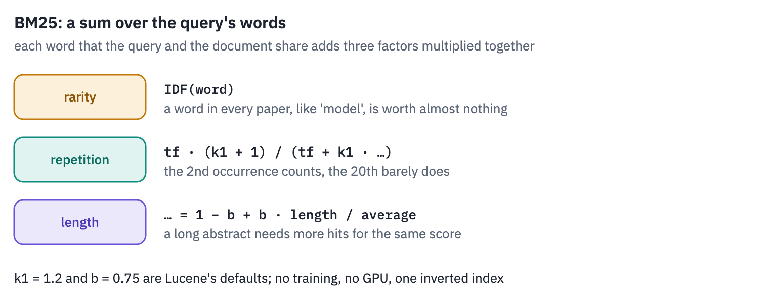
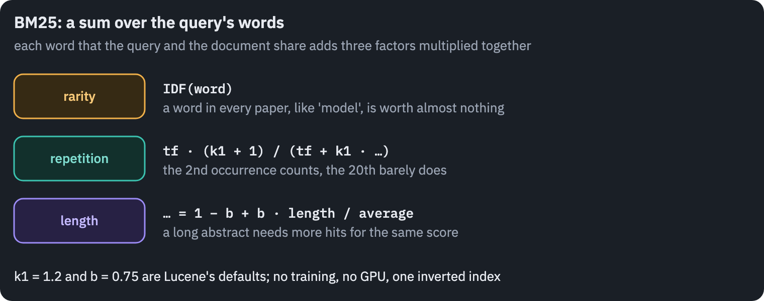
All three factors are common sense written down. A rare word says more than a common one. The second occurrence of a word matters, the twentieth adds almost nothing.
A long abstract mentions more words by sheer length, so it must mention them more often to score the same. The implementation is an inverted index: for every word, the documents that contain it and how often. A query then touches only the documents that share at least one of its words.
STOP = set("""a an and are as at be been by can for from has have in into is it its
of on or our such than that the their these they this to using was we were which
with""".split())


def words(text):
    return [w for w in re.findall(r"[a-z0-9]+", text.lower()) if w not in STOP]


class BM25:
    def __init__(self, texts, k1=1.2, b=0.75):
        self.k1 = k1
        postings = defaultdict(list)
        self.lengths = np.zeros(len(texts), dtype=np.float32)
        for doc, text in enumerate(texts):
            counts = Counter(words(text))
            self.lengths[doc] = sum(counts.values())
            for word, count in counts.items():
                postings[word].append((doc, count))
        self.index = {}
        for w, p in postings.items():
            docs, counts = zip(*p)
            self.index[w] = (np.array(docs), np.array(counts, dtype=np.float32))
        n = len(texts)
        self.idf = {w: math.log(1 + (n - len(d) + 0.5) / (len(d) + 0.5))
                    for w, (d, _) in self.index.items()}
        # the length part of the denominator, the same for every query
        self.norm = k1 * (1 - b + b * self.lengths / self.lengths.mean())

    def scores(self, query):
        out = np.zeros(len(self.lengths), dtype=np.float32)
        for w in set(words(query)):
            if w in self.index:
                docs, f = self.index[w]
                out[docs] += self.idf[w] * f * (self.k1 + 1) / (f + self.norm[docs])
        return out


start = time.time()
bm25 = BM25(texts)
postings = sum(len(docs) for docs, _ in bm25.index.values())
print(f"index: {len(bm25.index):,} words, {postings:,} postings, "
      f"built in {time.time() - start:.0f} s")
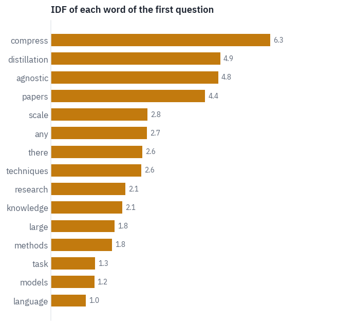
index: 107,892 words, 4,346,702 postings, built in 9 sHere is what BM25 thinks matters in the first question. Words like papers and methods occur in thousands of abstracts and weigh little; distillation and agnostic are rare and carry the query.
query = questions[0]
weights = {w: bm25.idf.get(w, 0.0) for w in dict.fromkeys(words(query))}
bars(dict(sorted(weights.items(), key=lambda kv: -kv[1])), fmt="{:.1f}",
     title="IDF of each word of the first question")
plt.show()

fig, ax = plt.subplots(figsize=(6.4, 3.4))
f = np.arange(0, 21)
for ratio, color in [(0.5, COLORS["enc"]), (1.0, COLORS["att"]), (2.0, COLORS["dec"])]:
    norm = 1.2 * (1 - 0.75 + 0.75 * ratio)
    ax.plot(f, f * 2.2 / (f + norm), color=color, marker="o", ms=3,
            label=f"document {ratio:g}× the average length")
ax.set_xlabel("occurrences of the word in the document")
ax.set_ylabel("multiplier of the word's IDF")
ax.set_title("Diminishing returns for repetition, a handicap for length")
ax.legend()
plt.show()
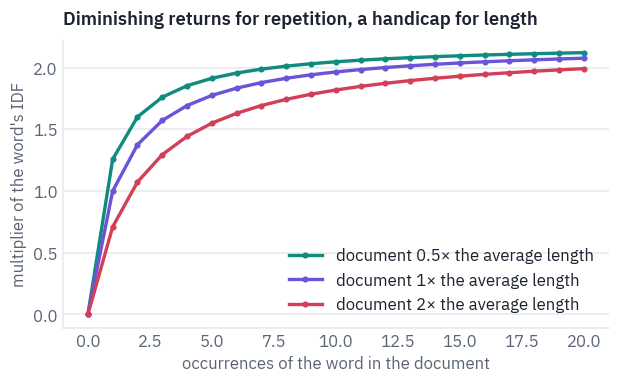
The multiplier can never exceed \(k_1 + 1 = 2.2\), however often the word repeats, and a document twice the average length needs about twice the occurrences to earn the same score. Now the search itself:
start = time.time()
bm25_scores = torch.from_numpy(np.stack([bm25.scores(q) for q in questions]))
evaluate("BM25", bm25_scores, time.time() - start, postings * 8)  # int32 id + float32 count
| method | recall@5 | recall@20 | ms per question | index, MB |
|---|---|---|---|---|
| BM25 | 0.45 | 0.60 | 1.03 | 34.77 |
With no training, no GPU and two parameters, BM25 puts the right paper in the top five for almost half the questions, a recall@5 of 0.45.
That is the number every model below has to beat, and the answer to anyone who says keyword search is dead.
3. An encoder’s own vectors: a crowd in a narrow cone
The obvious way to turn an encoder into a search engine is to average the vectors it computes for the tokens of a text and compare the averages by cosine.
Reimers and Gurevych tried it with BERT and found that it “yields rather bad sentence embeddings, often worse than averaging GloVe embeddings”. On their semantic similarity tests, averaged BERT vectors scored 54.8, BERT’s [CLS] vector 29.2, and plain averaged GloVe word vectors from 2014 scored 61.3. Let’s see why.
We take MiniLM-L6, a small encoder with BERT’s architecture. Microsoft distilled a 12-layer, 384-wide MiniLM from a larger model[4], and Nils Reimers, the same one, cut it to six layers by keeping every second layer.
It has five times fewer parameters than BERT-base, and, as section 5 will show, it is the starting point of the most popular embedding model there is. The BERT of the previous lessons loads it unchanged, once it learns to accept the segment ids that the cross-encoder of section 6 will need.
class Embeddings(nn.Module):
    def __init__(self, config):
        super().__init__()
        d = config["hidden_size"]
        self.words = nn.Embedding(config["vocab_size"], d)
        self.positions = nn.Embedding(config["max_position_embeddings"], d)
        self.segments = nn.Embedding(config["type_vocab_size"], d)
        self.norm = nn.LayerNorm(d, eps=config["layer_norm_eps"])
        self.dropout = nn.Dropout(config["hidden_dropout_prob"])

    def forward(self, ids, segments):
        positions = torch.arange(ids.shape[1], device=ids.device)
        x = self.words(ids) + self.positions(positions) + self.segments(segments)
        return self.dropout(self.norm(x))


class Layer(nn.Module):
    def __init__(self, config):
        super().__init__()
        d, eps = config["hidden_size"], config["layer_norm_eps"]
        self.heads = config["num_attention_heads"]
        self.q, self.k, self.v, self.out = (nn.Linear(d, d) for _ in range(4))
        self.norm1 = nn.LayerNorm(d, eps=eps)
        self.up = nn.Linear(d, config["intermediate_size"])
        self.down = nn.Linear(config["intermediate_size"], d)
        self.norm2 = nn.LayerNorm(d, eps=eps)
        self.dropout = nn.Dropout(config["hidden_dropout_prob"])

    def split(self, x):
        batch, length, d = x.shape
        return x.view(batch, length, self.heads, d // self.heads).transpose(1, 2)

    def forward(self, x, padding):
        q, k, v = self.split(self.q(x)), self.split(self.k(x)), self.split(self.v(x))
        scores = q @ k.transpose(-2, -1) / math.sqrt(q.shape[-1])
        lowest = torch.finfo(scores.dtype).min  # not -inf: a row of -inf turns into NaN
        scores = scores.masked_fill(padding[:, None, None, :], lowest)
        y = (self.dropout(scores.softmax(dim=-1)) @ v).transpose(1, 2).reshape(x.shape)
        x = self.norm1(x + self.dropout(self.out(y)))
        return self.norm2(x + self.dropout(self.down(F.gelu(self.up(x)))))


class Encoder(nn.Module):
    def __init__(self, config):
        super().__init__()
        self.embeddings = Embeddings(config)
        n_layers = config["num_hidden_layers"]
        self.layers = nn.ModuleList(Layer(config) for _ in range(n_layers))
        self.dim = config["hidden_size"]

    def forward(self, ids, padding, segments=None):
        segments = torch.zeros_like(ids) if segments is None else segments
        x = self.embeddings(ids, segments)
        for layer in self.layers:
            x = layer(x, padding)
        return x
Every model in this lesson is a BERT inside, and they store their tensors under the same names, with or without a bert. in front. One loader serves them all; whatever a checkpoint keeps besides the encoder, a pooler, a classifier or ColBERT’s projection, it returns separately.
PARTS = {"q": "attention.self.query", "k": "attention.self.key",
         "v": "attention.self.value", "out": "attention.output.dense",
         "norm1": "attention.output.LayerNorm", "up": "intermediate.dense",
         "down": "output.dense", "norm2": "output.LayerNorm"}


def bert_names(config):
    names = {"embeddings.words.weight": "embeddings.word_embeddings.weight",
             "embeddings.positions.weight": "embeddings.position_embeddings.weight",
             "embeddings.segments.weight": "embeddings.token_type_embeddings.weight",
             "embeddings.norm.weight": "embeddings.LayerNorm.weight",
             "embeddings.norm.bias": "embeddings.LayerNorm.bias"}
    for i in range(config["num_hidden_layers"]):
        for ours, theirs in PARTS.items():
            for p in ("weight", "bias"):
                names[f"layers.{i}.{ours}.{p}"] = f"encoder.layer.{i}.{theirs}.{p}"
    return names


def load_encoder(repo, file="model.safetensors"):
    with open(hf_hub_download(repo, "config.json")) as f:
        config = json.load(f)
    path = hf_hub_download(repo, file)
    if file.endswith(".safetensors"):
        weights = load_file(path)
    else:
        weights = torch.load(path, map_location="cpu", weights_only=True)
    prefix = "bert." if "bert.embeddings.word_embeddings.weight" in weights else ""
    encoder = Encoder(config)
    names = bert_names(config)
    encoder.load_state_dict({ours: weights[prefix + t] for ours, t in names.items()})
    used = {prefix + theirs for theirs in names.values()}
    extra = {k.removeprefix(prefix): v for k, v in weights.items()
             if k not in used and not k.endswith("position_ids")}
    return encoder.to(device).eval(), extra


BASE = "nreimers/MiniLM-L6-H384-uncased"
base, _ = load_encoder(BASE, "pytorch_model.bin")
tokenizer = AutoTokenizer.from_pretrained(BASE)
print(f"{sum(p.numel() for p in base.parameters()) / 1e6:.1f}M parameters")
22.6M parametersAn embedding of a text is one vector. We get it by mean pooling, averaging the token vectors while leaving out the padding, and normalise it to length one, so that the dot product of two embeddings is their cosine.
The papers are sorted by length before they are batched: a batch then pads to about the same length, and encoding runs about twice as fast.
def pool(hidden, padding, how):
    if how == "cls":
        return hidden[:, 0]
    keep = (~padding).unsqueeze(-1).to(hidden.dtype)
    return (hidden * keep).sum(1) / keep.sum(1)


@torch.no_grad()
def embed(encoder, texts, max_length, how="mean", prefix="", batch_size=128, tok=None):
    tok = tok or tokenizer
    order = np.argsort([-len(t) for t in texts])
    out = torch.empty(len(texts), encoder.dim, device=device)
    for start in range(0, len(texts), batch_size):
        rows = order[start:start + batch_size]
        batch = tok([prefix + texts[i] for i in rows], padding=True, truncation=True,
                    max_length=max_length, return_tensors="pt").to(device)
        padding = batch["attention_mask"] == 0
        with torch.autocast(device, dtype=torch.float16, enabled=device == "cuda"):
            hidden = encoder(batch["input_ids"], padding)
        vectors = pool(hidden.float(), padding, how)
        out[torch.as_tensor(rows, device=device)] = F.normalize(vectors, dim=-1)
    return out


def dense_search(name, encoder, how="mean", prefix="", tok=None):
    """Encode the corpus once, then every question, and score all papers by cosine."""
    docs = embed(encoder, texts, 256, how, tok=tok)
    start = time.time()
    found = embed(encoder, questions, 64, how, prefix, tok=tok) @ docs.T
    if device == "cuda":
        torch.cuda.synchronize()
    display(evaluate(name, found, time.time() - start, docs.numel() * 2))  # as float16
    return docs, found


start = time.time()
base_docs, base_scores = dense_search("MiniLM-L6, as pre-trained", base)
print(f"{len(texts):,} papers encoded in {time.time() - start:.0f} s")
| method | recall@5 | recall@20 | ms per question | index, MB |
|---|---|---|---|---|
| MiniLM-L6, as pre-trained | 0.00 | 0.00 | 0.29 | 44.53 |
57,986 papers encoded in 105 sNot one of the 593 questions finds its paper, not even in the top twenty. The histogram shows why: the cosines of random pairs of papers next to the cosines of questions with the papers they want.
def cosines(docs, found, n=4000):
    rng = torch.Generator().manual_seed(SEED)
    pairs = torch.randint(0, len(docs), (n, 2), generator=rng).to(device)
    random_pairs = (docs[pairs[:, 0]] * docs[pairs[:, 1]]).sum(1).cpu()
    right = torch.stack([found[i, wanted[0]] for i, wanted in enumerate(gold)]).cpu()
    return random_pairs, right


def cosine_histogram(ax, docs, found, title):
    random_pairs, right = cosines(docs, found)
    bins = np.linspace(-0.2, 1.0, 61)
    ax.hist(random_pairs, bins=bins, density=True, color=COLORS["line"], alpha=0.9,
            label="two random papers")
    ax.hist(right, bins=bins, density=True, color=COLORS["enc"], alpha=0.75,
            label="a question and its paper")
    ax.set_title(title)
    ax.set_xlabel("cosine")
    ax.set_yticks([])


fig, ax = plt.subplots(figsize=(6.4, 3.2))
cosine_histogram(ax, base_docs, base_scores, "MiniLM-L6 as pre-trained: all alike")
ax.legend(loc="upper left")
plt.show()
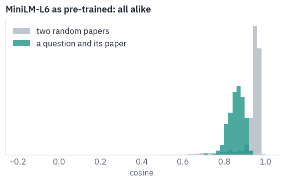
Two random abstracts have a cosine of about 0.95, and a question with the paper it asks for only about 0.85.
By this model’s measure a question is further from its own answer than any abstract is from any other abstract: the vectors say “this is an abstract” or “this is a question” much louder than what the text is about.
All of them crowd together. Ethayarajh (2019) found the same in almost every layer of BERT, ELMo and GPT-2: their representations are anisotropic, “occupying a narrow cone in the vector space” instead of spreading in all directions.
So what does it return? Here are the papers it puts first most often:
top5 = base_scores.topk(5, dim=1).indices
n_papers = top5.unique().numel()
print(f"{n_papers} different papers fill the top five of {len(questions)} questions")
for paper, count in Counter(top5.flatten().tolist()).most_common(3):
    name = re.sub(r"\s+", " ", titles[paper] or "(no title) " + texts[paper])
    print(f"{count:>4} questions get: {name[:72]}")
556 different papers fill the top five of 593 questions
  82 questions get: Why Neural Translations are the Right Length
  79 questions get: (no title) We detail methods for entity span identification and entity c
  70 questions get: Can language models capture syntactic associations without surface cues?
Most top fives differ, but a few papers turn up everywhere: Why Neural Translations are the Right Length is among the five best answers to 82 of the 593 questions, whatever they ask about. Such points sit near the middle of the crowd and are close to everything; retrieval people call them hubs.
Key point
Nothing in masked language modelling asked the model to put texts with similar meanings close together and the rest far apart; its vectors are good for the next layer, not for being compared with each other. To compare, the encoder has to be trained to compare.
4. Sentence-BERT: teaching an encoder to compare
Sentence-BERT’s architecture is a single encoder applied to each text separately, a bi-encoder (the paper calls it siamese), with mean pooling on top. All the novelty is in the training. In 2019 it learned from pairs of sentences labelled by people as entailment, contradiction or neutral, the SNLI and MultiNLI datasets.
Today the standard is contrastive training with in-batch negatives, which needs no labels at all, only pairs of texts that belong together: a question and its answer, a title and its abstract.
Google’s Smart Reply team put it in one sentence: “we use the responses of other examples in a training batch … as negative responses” [5], and Dense Passage Retrieval made the trick standard for search[6].
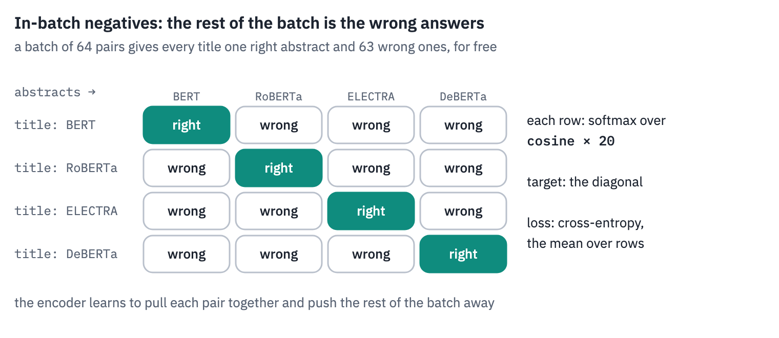
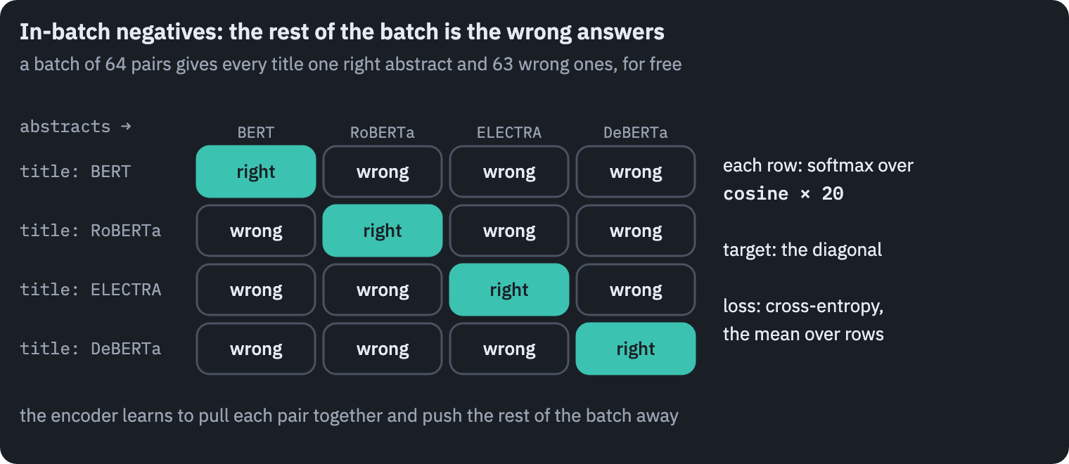
A batch holds \(B\) pairs \((t_i, a_i)\). Every title is compared with every abstract, and the loss asks each title to pick its own abstract out of the \(B\), as a classification with \(B\) classes:
\[\mathcal{L} = -\frac{1}{B} \sum_{i=1}^{B} \log \frac{\exp\left(s \cdot \cos(t_i, a_i)\right)}{\sum_{j=1}^{B} \exp\left(s \cdot \cos(t_i, a_j)\right)}\]This loss has many names: InfoNCE[7], the multiple negatives ranking loss, NT-Xent. The scale \(s = 20\), a temperature of 0.05, is what the sentence-transformers library uses by default: cosines live in \([-1, 1]\), and without the scale the softmax over them would be almost flat.
Our pairs are the titles and abstracts of the corpus itself, and that is the practical point. We use no question of LitSearch for training, only the papers we are going to search.
In practice
A company that wants search over its own documents rarely has thousands of labelled queries, but it always has documents, and documents have structure: titles and bodies, questions and answers in a support system, a function’s docstring and its code.
both = [i for i, (t, a) in enumerate(zip(titles, papers["abstract"])) if t and a.strip()]
pairs = [(titles[i], papers["abstract"][i]) for i in both]
BATCH, EPOCHS = (16, 1) if SMOKE else (128, 2)
steps = EPOCHS * (len(pairs) // BATCH)
if SMOKE:
    steps = 6
print(f"{len(pairs):,} title–abstract pairs, {steps:,} steps of {BATCH}")

student, _ = load_encoder(BASE, "pytorch_model.bin")


def pooled(model, texts, max_length):
    batch = tokenizer(texts, padding=True, truncation=True, max_length=max_length,
                      return_tensors="pt").to(device)
    padding = batch["attention_mask"] == 0
    with torch.autocast(device, dtype=torch.float16, enabled=device == "cuda"):
        hidden = model(batch["input_ids"], padding)
    return F.normalize(pool(hidden.float(), padding, "mean"), dim=-1)


def train_bi_encoder(model, scale=20.0, lr=5e-5, warmup=100):
    model.train()
    optimizer = torch.optim.AdamW(model.parameters(), lr=lr)
    schedule = torch.optim.lr_scheduler.LambdaLR(
        optimizer, lambda s: min(1.0, (s + 1) / warmup) * max(0.0, 1 - s / steps))
    scaler = torch.amp.GradScaler(enabled=device == "cuda")
    g = torch.Generator().manual_seed(SEED)
    order = torch.cat([torch.randperm(len(pairs), generator=g) for _ in range(EPOCHS)])
    log = []
    for step in range(steps):
        batch = [pairs[i] for i in order[step * BATCH:(step + 1) * BATCH]]
        t = pooled(model, [title for title, _ in batch], 32)
        a = pooled(model, [abstract for _, abstract in batch], 256)
        logits = scale * t @ a.T  # row i: title i against every abstract of the batch
        target = torch.arange(len(batch), device=device)
        loss = F.cross_entropy(logits, target)
        optimizer.zero_grad()
        scaler.scale(loss).backward()
        scaler.unscale_(optimizer)
        torch.nn.utils.clip_grad_norm_(model.parameters(), 1.0)
        scaler.step(optimizer)
        scaler.update()
        schedule.step()
        accuracy = (logits.argmax(1) == target).float().mean().item()
        log.append((loss.item(), accuracy))
    return model.eval(), np.array(log)


start = time.time()
student, log = train_bi_encoder(student)
print(f"trained in {time.time() - start:.0f} s")

fig, (left, right) = plt.subplots(1, 2, figsize=(8.4, 3.0))
window = max(1, len(log) // 40)
smooth = np.array([log[max(0, i - window):i + 1].mean(0) for i in range(len(log))])
left.plot(smooth[:, 0], color=COLORS["enc"])
left.set_title("loss")
right.plot(smooth[:, 1], color=COLORS["att"])
right.set_title(f"title finds its abstract among {BATCH}")
for ax in (left, right):
    ax.set_xlabel("step")
plt.show()
55,631 title–abstract pairs, 868 steps of 128
trained in 529 s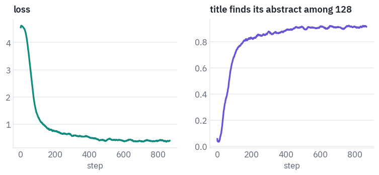
Within a few hundred steps a title finds its own abstract among 128 nine times out of ten. That is the training task; whether it carries over to questions the model has never seen is what the evaluation says.
student_docs, student_scores = dense_search("MiniLM-L6, trained here", student)
| method | recall@5 | recall@20 | ms per question | index, MB |
|---|---|---|---|---|
| MiniLM-L6, trained here | 0.32 | 0.46 | 0.25 | 44.53 |
From nothing to a third of the questions in ten minutes, without a single question in the training data. It is still well below BM25, and the reasons are plain: titles are not questions, and 55,000 pairs are not many.
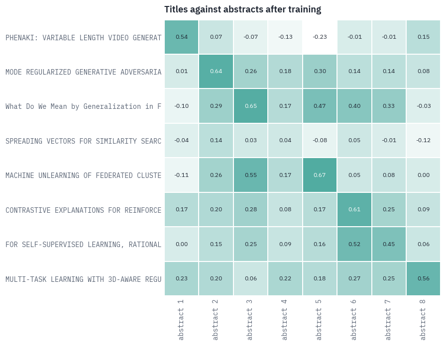
Here is the similarity matrix of eight papers the model trained on, as it looks after training. Six of the eight titles find their own abstract, on the diagonal. The misses are telling: SPREADING VECTORS FOR SIMILARITY SEARCH shares hardly a word with its abstract, which is about quantizers for indexing.
And the bright cells off the diagonal are not noise: the two papers on federated learning, rows 3 and 5, come out close to each other’s abstracts, which is what a search engine should want.
sample = both[:8]
short = [re.sub(r"\s+", " ", titles[i])[:38] for i in sample]
with torch.no_grad():
    t = pooled(student, [titles[i] for i in sample], 32)
    a = pooled(student, [papers["abstract"][i] for i in sample], 256)
heatmap((t @ a.T).cpu().numpy(), rows=short, cols=[f"abstract {k + 1}" for k in range(8)],
        annotate=True, fmt="{:.2f}", cell=0.62, vmin=-0.2, vmax=1.0, role="enc",
        title="Titles against abstracts after training")
plt.show()

fig, axes = plt.subplots(1, 2, figsize=(8.8, 3.0), sharex=True)
cosine_histogram(axes[0], base_docs, base_scores, "before")
cosine_histogram(axes[1], student_docs, student_scores, "after training on our pairs")
axes[0].legend(loc="upper left", fontsize=8)
plt.show()
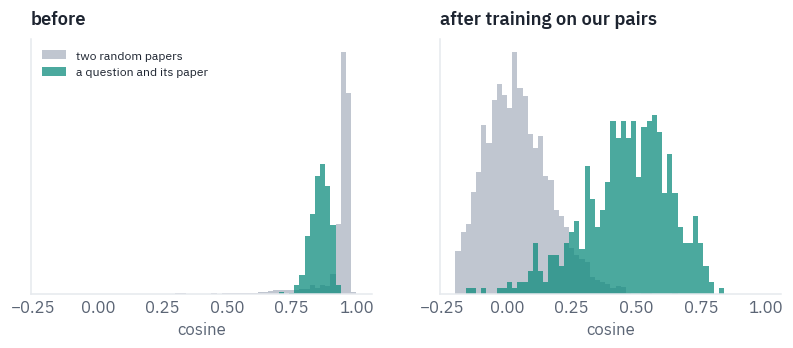
The cone has opened. Random pairs of papers now spread around zero, and the questions, which the model never saw during training, sit to the right of them, around 0.5. The model learned what makes two texts in this corpus mean the same thing, from the corpus alone.
5. What a billion pairs buy
all-MiniLM-L6-v2 is not just the most popular embedding model: with 184 million downloads in the month before this lesson was written, it is the most downloaded model of any kind on the Hugging Face Hub.
Its model card says it started from exactly our nreimers/MiniLM-L6-H384-uncased and was trained with the same loss, on 1,170,060,424 pairs from 290 sources: Reddit, Stack Exchange, WikiAnswers, PAQ, and 41,769,185 titles with their abstracts from the S2ORC corpus of scientific papers, which is our task at 750 times our scale. It trained for 100,000 steps of 1,024 pairs on a TPU v3-8.
Same architecture, same starting point, same loss; only the data differ. So the comparison with our model shows what the data buy. Its weights load into our code, and the check against Hugging Face’s BertModel:
MINILM = "sentence-transformers/all-MiniLM-L6-v2"
minilm, _ = load_encoder(MINILM)
reference = BertModel.from_pretrained(MINILM).to(device).eval()
check = tokenizer(questions[:4], padding=True, return_tensors="pt").to(device)
padding = check["attention_mask"] == 0
with torch.no_grad():
    theirs = reference(**check).last_hidden_state
    ours = minilm(check["input_ids"], padding)
gap = (ours - theirs)[~padding].abs().max().item()
print(f"largest difference from Hugging Face: {gap:.1e}")
assert gap < 1e-3
del reference

minilm_docs, minilm_scores = dense_search("all-MiniLM-L6-v2", minilm)
largest difference from Hugging Face: 1.8e-06| method | recall@5 | recall@20 | ms per question | index, MB |
|---|---|---|---|---|
| all-MiniLM-L6-v2 | 0.42 | 0.59 | 0.25 | 44.53 |
Ten points above our ten-minute model, and still three below BM25: 750 times more of our task, and a billion other pairs, bought ten points. Before going further, one more thing that costs nothing to check. The model was trained with mean pooling; here it is read with the [CLS] vector instead, the other common choice:
_ = dense_search("all-MiniLM-L6-v2, [CLS] instead of the mean", minilm, "cls")
| method | recall@5 | recall@20 | ms per question | index, MB |
|---|---|---|---|---|
| all-MiniLM-L6-v2, [CLS] instead of the mean | 0.30 | 0.43 | 0.25 | 44.53 |
Trap
Twelve points gone, without an error or a warning: the vectors look like vectors, and the search still works, only worse. A model is its weights and its pooling, and the card says which pooling.
The most practical question of the section is the next one. We have a general model trained on a billion pairs, and a corpus with 55,000 pairs of its own. Does a few minutes of the same training on our titles and abstracts, starting from all-MiniLM-L6-v2 instead of from scratch, adapt it to this corpus?
adapted, _ = load_encoder(MINILM)
start = time.time()
adapted, adapted_log = train_bi_encoder(adapted, lr=2e-5)
found = adapted_log[-50:, 1].mean()
print(f"adapted in {time.time() - start:.0f} s; in the last 50 steps a title found "
      f"its abstract {found:.0%} of the time")
adapted_docs, adapted_scores = dense_search("all-MiniLM-L6-v2, adapted here", adapted)
adapted in 527 s; in the last 50 steps a title found its abstract 97% of the time| method | recall@5 | recall@20 | ms per question | index, MB |
|---|---|---|---|---|
| all-MiniLM-L6-v2, adapted here | 0.51 | 0.65 | 0.25 | 44.53 |
Ten minutes of the same training took all-MiniLM-L6-v2 from 0.42 to 0.51, above BM25.
The general model brought what a billion pairs teach about language; our pairs showed it what this corpus’s titles and abstracts look like. This is the cheapest improvement in the lesson, and it is open to anyone with a corpus: no labels, no questions, one T4.
BGE models from the Beijing Academy of Artificial Intelligence are a newer generation of the same idea [8]: BERT’s architecture again, with pre-training aimed at retrieval, contrastive training on a larger and cleaner collection, and a final round on labelled data.
The base size has 12 layers and 768 dimensions. Its model card says two things that are easy to miss: the embedding is the vector of [CLS], not the mean, and a query, though not a document, should start with an instruction; without it, the card promises “a slight degradation”.
BGE = "BAAI/bge-base-en-v1.5"
INSTRUCTION = "Represent this sentence for searching relevant passages: "
bge, _ = load_encoder(BGE)
bge_tokenizer = AutoTokenizer.from_pretrained(BGE)
bge_docs, bge_scores = dense_search("bge-base-en-v1.5", bge, "cls", INSTRUCTION,
                                   tok=bge_tokenizer)
_ = dense_search("bge-base-en-v1.5, mean pooling, no instruction", bge,
                 tok=bge_tokenizer)
| method | recall@5 | recall@20 | ms per question | index, MB |
|---|---|---|---|---|
| bge-base-en-v1.5 | 0.50 | 0.67 | 0.83 | 89.07 |
| method | recall@5 | recall@20 | ms per question | index, MB |
|---|---|---|---|---|
| bge-base-en-v1.5, mean pooling, no instruction | 0.51 | 0.66 | 0.71 | 89.07 |
bge-base-en-v1.5, with twice the layers and twice the width, scores 0.50: the same as the small model adapted to our corpus, with an index twice the size and three times the time per question. The second line holds a surprise.
Used against its card’s advice, with mean pooling and no instruction, bge does no worse. Its card warns only of “a slight degradation” without the instruction, and here even that is lost in the noise, while all-MiniLM-L6-v2 read with [CLS] lost twelve points. Pooling matters for one model and not for another, and you can’t know which without checking.
table(pd.DataFrame(results))
| method | recall@5 | recall@20 | ms per question | index, MB |
|---|---|---|---|---|
| BM25 | 0.45 | 0.60 | 1.03 | 34.77 |
| MiniLM-L6, as pre-trained | 0.00 | 0.00 | 0.29 | 44.53 |
| MiniLM-L6, trained here | 0.32 | 0.46 | 0.25 | 44.53 |
| all-MiniLM-L6-v2 | 0.42 | 0.59 | 0.25 | 44.53 |
| all-MiniLM-L6-v2, [CLS] instead of the mean | 0.30 | 0.43 | 0.25 | 44.53 |
| all-MiniLM-L6-v2, adapted here | 0.51 | 0.65 | 0.25 | 44.53 |
| bge-base-en-v1.5 | 0.50 | 0.67 | 0.83 | 89.07 |
| bge-base-en-v1.5, mean pooling, no instruction | 0.51 | 0.66 | 0.71 | 89.07 |
6. The cross-encoder: reading the question and the paper together
A bi-encoder never sees the query and the document at the same time; it compares two summaries written independently.
A cross-encoder is plain BERT reading a pair of texts, in the input format of lesson 1: the query and the document go in as one sequence, [CLS] query [SEP] document [SEP], the two parts marked by their segment ids, and every token of the query attends to every token of the document in every layer.
On top sits a classifier that turns the [CLS] vector into one number, a relevance score.
Putting BERT on top of BM25 this way was one of the first places where BERT took over search [9]. It is the most accurate of the three architectures and the most expensive: nothing can be computed before the query arrives.
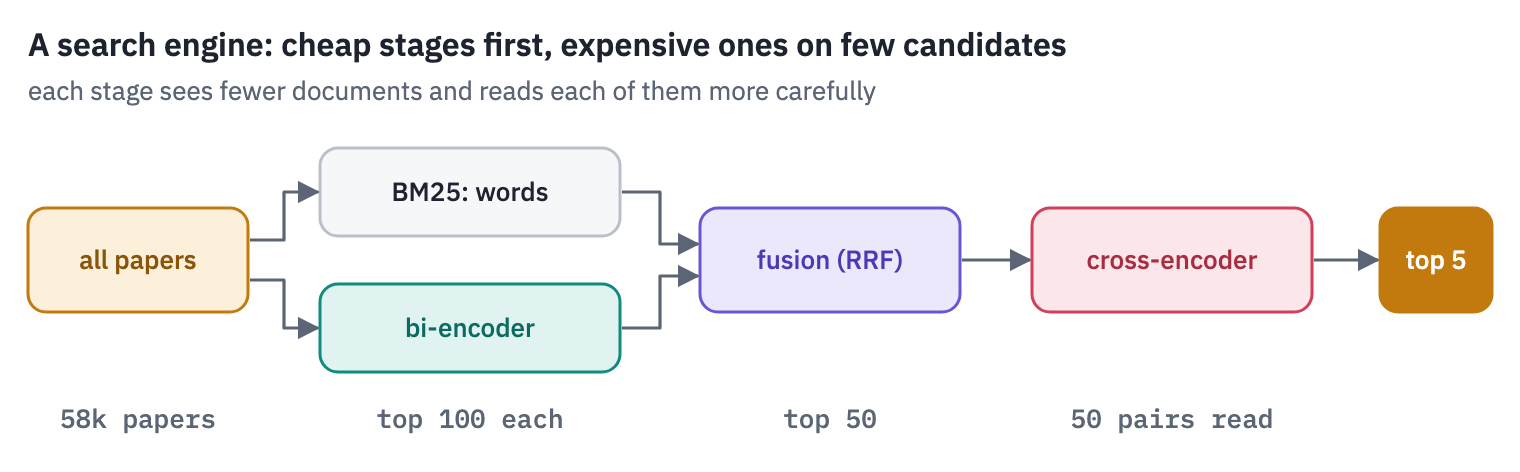
Scoring all 58,000 papers for one question would take 58,000 passes of the encoder. So a cross-encoder is used as a reranker: a fast retriever proposes a few dozen candidates and the cross-encoder reorders them.
We take cross-encoder/ms-marco-MiniLM-L6-v2, the same six-layer MiniLM trained on MS MARCO: real Bing queries, each with the passages that human editors marked as containing the answer. Besides the encoder it has BERT’s pooler, a dense layer with tanh on the [CLS] vector, and the classifier with a single output.
class CrossEncoder(nn.Module):
    def __init__(self, repo):
        super().__init__()
        self.encoder, extra = load_encoder(repo)
        d = self.encoder.dim
        self.pooler, self.classifier = nn.Linear(d, d), nn.Linear(d, 1)
        self.pooler.load_state_dict({"weight": extra["pooler.dense.weight"],
                                     "bias": extra["pooler.dense.bias"]})
        self.classifier.load_state_dict({"weight": extra["classifier.weight"],
                                         "bias": extra["classifier.bias"]})

    def forward(self, ids, padding, segments):
        hidden = self.encoder(ids, padding, segments)
        return self.classifier(torch.tanh(self.pooler(hidden[:, 0]))).squeeze(-1)


RERANKER = "cross-encoder/ms-marco-MiniLM-L6-v2"
reranker = CrossEncoder(RERANKER).to(device).eval()
reranker_tokenizer = AutoTokenizer.from_pretrained(RERANKER)
# the reference reads the PyTorch file: this model's safetensors file keeps its tensors at
# offsets that aren't multiples of four bytes; Apple's CPU math library returns NaN there
reference = AutoModelForSequenceClassification.from_pretrained(RERANKER,
                                                               use_safetensors=False)
reference = reference.to(device).eval()
pair = reranker_tokenizer([questions[0]] * 2, [texts[gold[0][0]], texts[0]], padding=True,
                          truncation=True, max_length=256, return_tensors="pt").to(device)
with torch.no_grad():
    theirs = reference(**pair).logits.squeeze(-1)
    ours = reranker(pair["input_ids"], pair["attention_mask"] == 0, pair["token_type_ids"])
print("Hugging Face:", theirs.cpu().numpy().round(3), " ours:", ours.cpu().numpy().round(3))
assert (ours - theirs).abs().max() < 1e-3
del reference
print(reranker_tokenizer.convert_ids_to_tokens(pair["input_ids"][0])[:24])
Hugging Face: [ 1.074 -9.094]  ours: [ 1.074 -9.094]
['[CLS]', 'are', 'there', 'any', 'research', 'papers', 'on', 'methods', 'to', 'com', '##press', 'large', '-', 'scale', 'language', 'models', 'using', 'task', '-', 'ag', '##nostic', 'knowledge', 'di', '##sti']
The first pair is the first question with the paper it wants, the second the same question with a random paper: the scores are logits, and only their order matters. The reranker takes the top 50 papers of a first-stage search and replaces their scores with its own; everything below the 50 stays below.
@torch.no_grad()
def rerank(name, scores, depth=50, max_length=320):
    start = time.time()
    candidates = scores.topk(depth, dim=1).indices
    reranked = torch.full_like(scores, -1e4)
    for i, question in enumerate(questions):
        docs = candidates[i].tolist()
        batch = reranker_tokenizer([question] * depth, [texts[j] for j in docs],
                                   padding=True, truncation="only_second",
                                   max_length=max_length, return_tensors="pt").to(device)
        with torch.autocast(device, dtype=torch.float16, enabled=device == "cuda"):
            logits = reranker(batch["input_ids"], batch["attention_mask"] == 0,
                              batch["token_type_ids"])
        reranked[i, candidates[i]] = logits.float()
    seconds = time.time() - start
    display(evaluate(name, reranked, seconds, 0))
    return reranked


reranked_minilm = rerank("all-MiniLM-L6-v2 → reranker", minilm_scores.to(device))
| method | recall@5 | recall@20 | ms per question | index, MB |
|---|---|---|---|---|
| all-MiniLM-L6-v2 → reranker | 0.54 | 0.64 | 131.45 | 0.00 |
The reranker lifts all-MiniLM-L6-v2 from 0.42 to 0.54: reading each of the 50 candidates together with the question, it puts the right paper in the first five for about 70 more questions.
It also takes 131 ms per question, five hundred times as long as the search that found the candidates. That is the trade a reranker always offers.
7. ColBERT: a vector for every token
Between the two extremes sits late interaction, from Omar Khattab and Matei Zaharia at Stanford [10]. Like a bi-encoder, ColBERT encodes the query and the document separately, so the documents can be indexed in advance.
Unlike it, ColBERT keeps a vector for every token, shrunk by a linear layer from 768 dimensions to 128 and normalised.
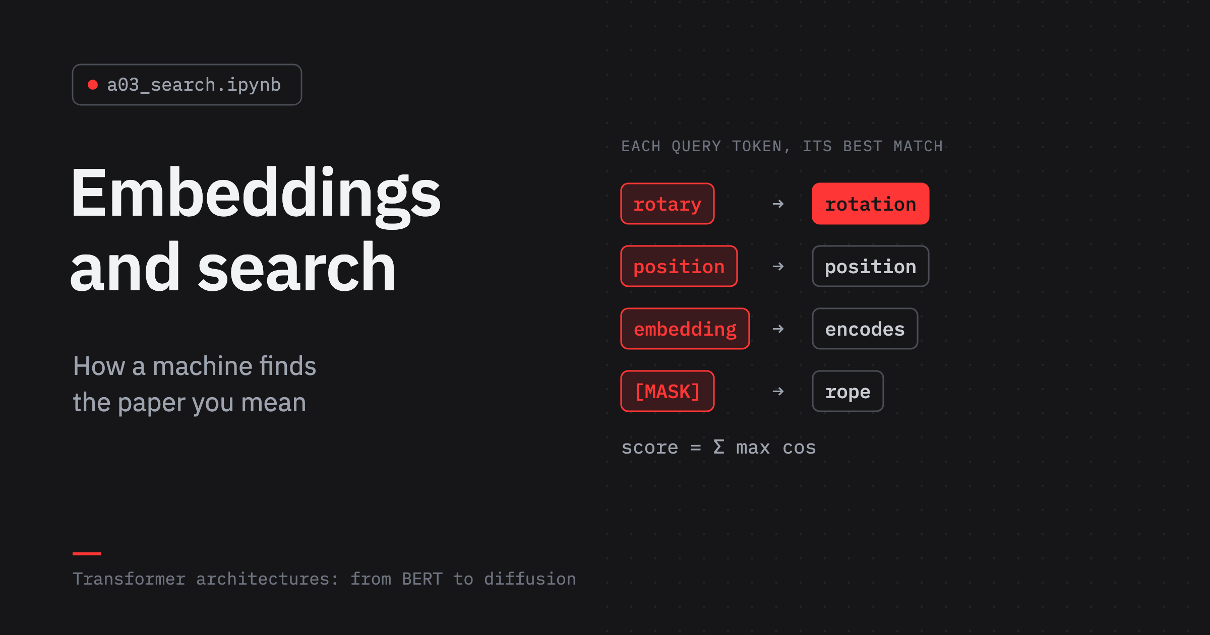
The query and the document meet only at the very end, in MaxSim: every query token finds the document token most similar to it, and the document’s score is the sum of these best matches. Against a BERT reranker, the paper reported search “two orders-of-magnitude faster and requiring four orders-of-magnitude fewer FLOPs per query”.
\[\text{score}(q, d) = \sum_{i \in q} \max_{j \in d} \cos(q_i, d_j)\]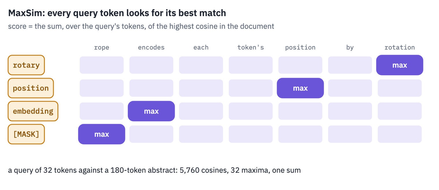
A few details matter for loading the real model, ColBERTv2 [11]. The encoder is BERT-base. The query starts with a marker token after [CLS], and the document with another; ColBERT’s code writes them into BERT’s unused vocabulary slots, [unused0] and [unused1].
A query is always 32 tokens long: what the question doesn’t fill is padded with [MASK], the model doesn’t attend to these masks, but their output vectors still take part in MaxSim.
The paper calls this query augmentation: the masks become soft extra query terms that the model fills with whatever the question implies. Document tokens that are punctuation are dropped from the index.
class ColBERT(nn.Module):
    def __init__(self, repo):
        super().__init__()
        self.encoder, extra = load_encoder(repo)
        self.linear = nn.Linear(self.encoder.dim, 128, bias=False)
        self.linear.load_state_dict({"weight": extra["linear.weight"]})

    def forward(self, ids, padding):
        return F.normalize(self.linear(self.encoder(ids, padding)), dim=-1)


COLBERT = "colbert-ir/colbertv2.0"
colbert = ColBERT(COLBERT).to(device).eval()
colbert_tokenizer = AutoTokenizer.from_pretrained(COLBERT)
Q_MARKER, D_MARKER = colbert_tokenizer.convert_tokens_to_ids(["[unused0]", "[unused1]"])
punctuation = colbert_tokenizer.convert_tokens_to_ids(list(string.punctuation))
PUNCTUATION = torch.tensor(punctuation, device=device)

reference = BertModel.from_pretrained(COLBERT).to(device).eval()
check = colbert_tokenizer(questions[:4], padding=True, return_tensors="pt").to(device)
padding = check["attention_mask"] == 0
with torch.no_grad():
    theirs = reference(**check).last_hidden_state
    ours = colbert.encoder(check["input_ids"], padding)
gap = (ours - theirs)[~padding].abs().max().item()
print(f"ColBERTv2's encoder, largest difference from Hugging Face: {gap:.1e}")
assert gap < 1e-3
del reference


@torch.no_grad()
def colbert_queries(texts, length=32):
    batch = colbert_tokenizer([". " + t for t in texts], padding="max_length",
                              truncation=True, max_length=length,
                              return_tensors="pt").to(device)
    ids, attended = batch["input_ids"], batch["attention_mask"]
    ids[:, 1] = Q_MARKER  # the original ColBERT code's trick: ". " held the marker's place
    ids[ids == colbert_tokenizer.pad_token_id] = colbert_tokenizer.mask_token_id
    with torch.autocast(device, dtype=torch.float16, enabled=device == "cuda"):
        return colbert(ids, attended == 0).to(half), ids


@torch.no_grad()
def colbert_documents(texts, length=180):
    batch = colbert_tokenizer([". " + t for t in texts], padding=True, truncation=True,
                              max_length=length, return_tensors="pt").to(device)
    ids, attended = batch["input_ids"], batch["attention_mask"]
    ids[:, 1] = D_MARKER
    with torch.autocast(device, dtype=torch.float16, enabled=device == "cuda"):
        vectors = colbert(ids, attended == 0)
    keep = (attended == 1) & ~torch.isin(ids, PUNCTUATION)
    return (vectors * keep.unsqueeze(-1)).to(half), keep, ids
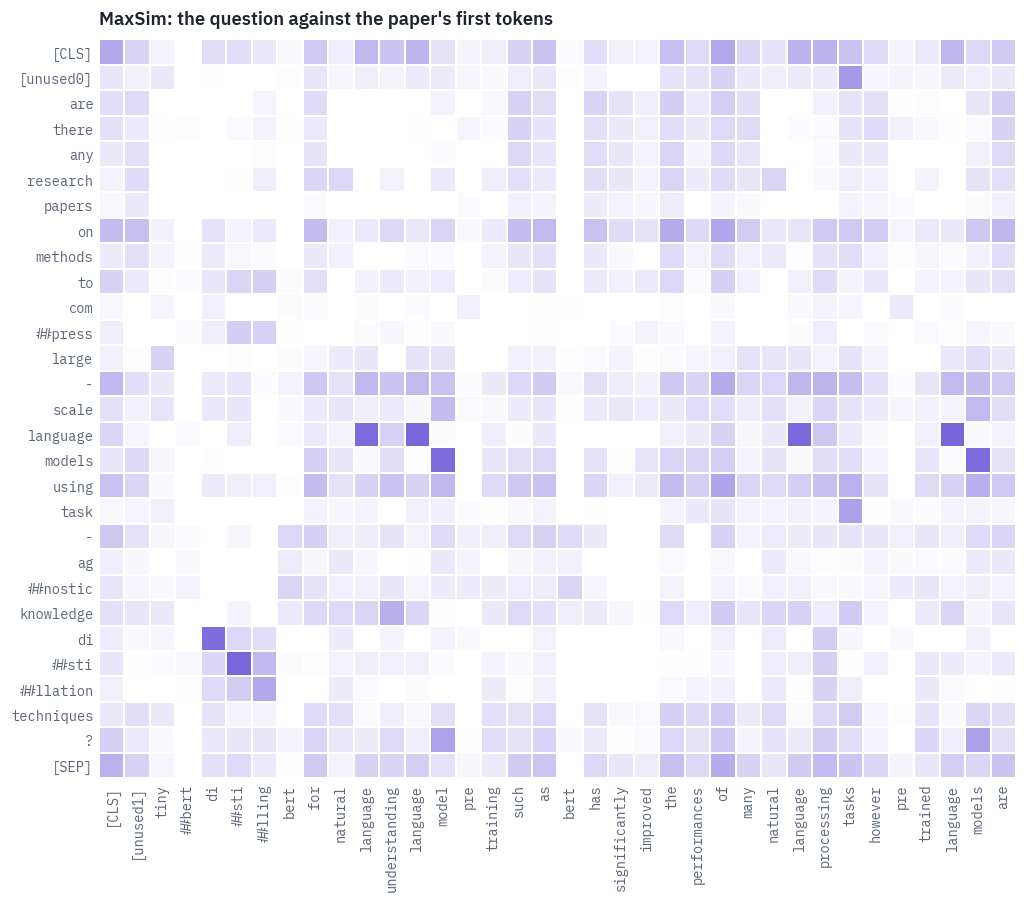
ColBERTv2's encoder, largest difference from Hugging Face: 2.1e-06Before indexing anything, here is MaxSim at work on the first question and the paper it wants. Each row is a token of the question, each column a token of the abstract; the brightest cell of a row is the match that row contributes.
q_vectors, q_ids = colbert_queries(questions[:1])
d_vectors, d_keep, d_ids = colbert_documents([texts[gold[0][0]]])
q_tokens = colbert_tokenizer.convert_ids_to_tokens(q_ids[0])
d_tokens = colbert_tokenizer.convert_ids_to_tokens(d_ids[0])
shown = [j for j in range(len(d_tokens)) if d_keep[0, j]][:36]
n_words = q_tokens.index("[SEP]") + 1
similarity = (q_vectors[0, :n_words].float() @ d_vectors[0, shown].float().T).cpu().numpy()
heatmap(similarity, rows=q_tokens[:n_words], cols=[d_tokens[j] for j in shown], cell=0.26,
        vmin=0.0, vmax=1.0, title="MaxSim: the question against the paper's first tokens")
plt.show()
print("best match of each question token:")
print(", ".join(f"{q}→{d_tokens[shown[j]]}" for q, j in zip(q_tokens[2:n_words - 1],
                                                          similarity.argmax(1)[2:-1])))
best match of each question token:
are→the, there→are, any→the, research→natural, papers→[unused1], on→of, methods→of, to→of, com→pre, ##press→##sti, large→tiny, -→of, scale→models, language→language, models→models, using→of, task→tasks, -→[CLS], ag→natural, ##nostic→bert, knowledge→understanding, di→di, ##sti→##sti, ##llation→##lling, techniques→of, ?→models
Most question tokens find their namesakes, piece by piece: di, ##sti, ##llation find the di, ##sti, ##lling of TinyBERT: Distilling BERT, and language and models find themselves.
Some matches are about meaning rather than spelling: large finds tiny. The question’s filler words, are, there, on, to, settle for whatever filler is nearest; they add a little to every paper’s score and decide nothing.
Now the whole corpus. The index keeps up to 180 vectors of 128 numbers for every paper. On a GPU we can afford to search it exhaustively: for every question, MaxSim against every paper, in blocks.
start = time.time()
order = np.argsort([-len(t) for t in texts])
index = torch.zeros(len(texts), 180, 128, dtype=half, device=device)
n_vectors = 0
for s in range(0, len(texts), 128):
    rows = order[s:s + 128]
    vectors, keep, _ = colbert_documents([texts[i] for i in rows])
    index[torch.as_tensor(rows, device=device), :vectors.shape[1]] = vectors
    n_vectors += keep.sum().item()
print(f"indexed in {time.time() - start:.0f} s: {n_vectors:,} vectors, "
      f"{n_vectors / len(texts):.0f} per paper")


@torch.no_grad()
def maxsim_search(query_vectors, block=2048):
    scores = torch.empty(len(query_vectors), len(index), device=device)
    for qs in range(0, len(query_vectors), 16):
        q = query_vectors[qs:qs + 16]
        for ds in range(0, len(index), block):
            sim = torch.einsum("aqd,nld->anql", q, index[ds:ds + block])
            scores[qs:qs + 16, ds:ds + block] = sim.amax(-1).float().sum(-1)
    return scores


start = time.time()
colbert_scores = maxsim_search(colbert_queries(questions)[0])
if device == "cuda":
    torch.cuda.synchronize()
evaluate("ColBERTv2", colbert_scores, time.time() - start, n_vectors * 128 * 2)
indexed in 209 s: 7,982,607 vectors, 138 per paper| method | recall@5 | recall@20 | ms per question | index, MB |
|---|---|---|---|---|
| ColBERTv2 | 0.47 | 0.62 | 13.77 | 2,043.55 |
ColBERTv2 lands between the small and the large single-vector models: 0.47, above BM25 and all-MiniLM-L6-v2, below bge and the adapted MiniLM. Its price is the index, eight million vectors and 2 GB in float16, more than twenty times bge’s, and 14 ms per question even on a GPU.
Like the reranker, it learned what relevant means from MS MARCO’s web queries, not from questions about papers.
8. A search engine
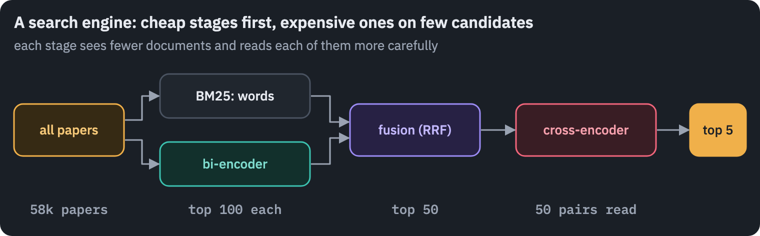
Each method has seen the questions its own way, and their mistakes differ. BM25 cannot know that compressing a model and distillation are related; an embedding can miss that the question names a specific dataset.
The simplest way to combine rankings is reciprocal rank fusion[12]: each paper gets \(\sum_r 1 / (60 + \text{rank}_r)\) over the rankings \(r\) that contain it. It needs no training and no calibration of scores, which is the point: BM25’s scores and cosines are on scales that have nothing to do with each other, and ranks are on the same scale by construction.
def fuse(*rankings, k=60, depth=100):
    fused = torch.zeros_like(rankings[0])
    weight = 1 / (k + torch.arange(1, depth + 1, device=fused.device, dtype=fused.dtype))
    for scores in rankings:
        top = scores.topk(depth, dim=1).indices
        fused.scatter_add_(1, top, weight.expand_as(top).contiguous())
    return fused


bm25_gpu = bm25_scores.to(device)
for name, scores in [("MiniLM-L6, trained here", student_scores),
                     ("all-MiniLM-L6-v2", minilm_scores),
                     ("all-MiniLM-L6-v2, adapted here", adapted_scores),
                     ("bge-base-en-v1.5", bge_scores)]:
    evaluate(f"BM25 + {name}", fuse(bm25_gpu, scores), 0, 0)
hybrid = fuse(bm25_gpu, adapted_scores)
reranked = rerank("BM25 + MiniLM adapted → reranker", hybrid)
engine_scores = fuse(hybrid, reranked, depth=50)  # the reranker's order and the hybrid's
evaluate("BM25 + MiniLM adapted + reranker, fused", engine_scores, 0, 0)
table(pd.DataFrame(results).drop(columns=["ms per question", "index, MB"]))
| method | recall@5 | recall@20 | ms per question | index, MB |
|---|---|---|---|---|
| BM25 + MiniLM adapted → reranker | 0.55 | 0.71 | 132.62 | 0.00 |
| method | recall@5 | recall@20 |
|---|---|---|
| BM25 | 0.45 | 0.60 |
| MiniLM-L6, as pre-trained | 0.00 | 0.00 |
| MiniLM-L6, trained here | 0.32 | 0.46 |
| all-MiniLM-L6-v2 | 0.42 | 0.59 |
| all-MiniLM-L6-v2, [CLS] instead of the mean | 0.30 | 0.43 |
| all-MiniLM-L6-v2, adapted here | 0.51 | 0.65 |
| bge-base-en-v1.5 | 0.50 | 0.67 |
| bge-base-en-v1.5, mean pooling, no instruction | 0.51 | 0.66 |
| all-MiniLM-L6-v2 → reranker | 0.54 | 0.64 |
| ColBERTv2 | 0.47 | 0.62 |
| BM25 + MiniLM-L6, trained here | 0.47 | 0.63 |
| BM25 + all-MiniLM-L6-v2 | 0.53 | 0.68 |
| BM25 + all-MiniLM-L6-v2, adapted here | 0.56 | 0.70 |
| BM25 + bge-base-en-v1.5 | 0.55 | 0.69 |
| BM25 + MiniLM adapted → reranker | 0.55 | 0.71 |
| BM25 + MiniLM adapted + reranker, fused | 0.59 | 0.73 |
Fusion is the best deal in the table. BM25 + all-MiniLM-L6-v2 reaches 0.53, eleven points above the model alone and eight above BM25, from two rankings that each find what the other misses. Even our ten-minute model, at 0.32 on its own, lifts BM25 by two points.
With the adapted MiniLM the hybrid reaches 0.56, as much as bge with BM25. The reranker on top of that hybrid changes nothing at five: on candidates this good, its judgement, learned from Bing queries, is no better than the hybrid’s.
Fused with the hybrid’s order, the two judgements together give the best result of the lesson, 0.59 at five and 0.73 at twenty.
Fusion and reranking add no index of their own, so their cost in the table is the cost of their parts. The whole picture, quality against the time a question takes and the memory its index needs:
frame = pd.DataFrame(results).set_index("method")
single = ["BM25", "MiniLM-L6, trained here", "all-MiniLM-L6-v2",
          "all-MiniLM-L6-v2, adapted here", "bge-base-en-v1.5", "ColBERTv2"]
points = {name: frame.loc[name] for name in single}
parts = frame.loc[["BM25", "all-MiniLM-L6-v2, adapted here",
                   "BM25 + MiniLM adapted → reranker"]].sum()
engine = "BM25 + MiniLM adapted + reranker, fused"
points["the search engine"] = pd.Series({"recall@5": frame.loc[engine, "recall@5"],
                                         "ms per question": parts["ms per question"],
                                         "index, MB": parts["index, MB"]})

fig, (left, right) = plt.subplots(1, 2, figsize=(9.6, 3.8), sharey=True)
for name, row in points.items():
    special = {"BM25": COLORS["data"], "the search engine": COLORS["att"]}
    color = special.get(name, COLORS["enc"])
    for ax, x in ((left, row["ms per question"]), (right, row["index, MB"])):
        ax.scatter(x, row["recall@5"], s=55, color=color, zorder=3)
        left_side = name in ("all-MiniLM-L6-v2, adapted here", "BM25")
        ax.annotate(name, (x, row["recall@5"]), xytext=(-6 if left_side else 6, 4),
                    textcoords="offset points", fontsize=8,
                    ha="right" if left_side else "left")
for ax in (left, right):
    ax.set_xscale("log")
    ax.margins(x=0.3)
left.set_xlabel("milliseconds per question, log scale")
right.set_xlabel("index size, MB, log scale")
left.set_ylabel("recall@5")
left.set_title("Quality against time")
right.set_title("Quality against memory")
plt.show()
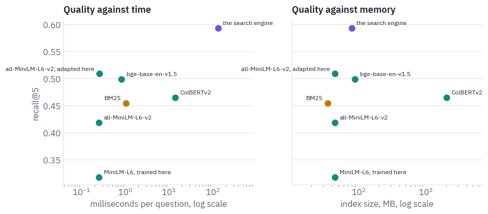
The search engine is alone at the top of both charts. Almost all of its time is the reranker’s, about 130 ms per question on a T4; everything else answers in a millisecond or less, except ColBERT, which also needs twenty times the memory of anything else here.
Where the methods disagree is more instructive than the averages. For every question we find the rank of its first right paper under BM25 and under the adapted MiniLM, and look at the questions where one of them finds the paper at once and the other buries it.
def first_rank(scores):
    order = scores.argsort(dim=1, descending=True).cpu().numpy()
    position = np.empty_like(order)
    position[np.arange(len(order))[:, None], order] = np.arange(order.shape[1])
    return np.array([min(position[i, g]) + 1 for i, g in enumerate(gold)])


ranks = pd.DataFrame({"question": questions, "BM25": first_rank(bm25_gpu),
                      "MiniLM": first_rank(adapted_scores),
                      "engine": first_rank(engine_scores)})
words_win = ranks[(ranks["BM25"] <= 3) & (ranks["MiniLM"] > 50)]
meaning_wins = ranks[(ranks["MiniLM"] <= 3) & (ranks["BM25"] > 50)]
print(f"BM25 in the top 3, MiniLM below 50: {len(words_win)} questions; "
      f"the other way round: {len(meaning_wins)}")
display(table(pd.concat([words_win.head(3), meaning_wins.head(3)])))
BM25 in the top 3, MiniLM below 50: 13 questions; the other way round: 22| question | BM25 | MiniLM | engine |
|---|---|---|---|
| In the context of natural language processing, I am looking for research that explores the relationship between a model's prediction entropy and its tendencies to copy existing text versus generating novel content. Can you recommend a paper? | 1 | 162 | 3 |
| How to achieve zero-shot lip reading? | 1 | 187 | 4 |
| Is there any work that allows large numbers of model outputs to be encoded and compared by causal language models in a single forward pass? | 3 | 846 | 3 |
| Can you recommend a conversational QA dataset where the human questioner does not have access to the evidence passage to simulate a more real-world information-seeking environment? | 155 | 2 | 23 |
| Can you suggest any literature that explores the idea of training neural networks to translate text passages into related questions? | 100 | 1 | 4 |
| When using pretrained transformer models for generating sentence embeddings, I've heard different strategies such as mean pooling and using the CLS token's embedding. What study shows that mean pooling outperforms CLS in semantic similarity tasks? | 59 | 3 | 16 |
BM25 wins when a question hangs on a rare, exact term: zero-shot lip reading, prediction entropy, a single forward pass. The adapted model wins on paraphrase: the question about networks that “translate text passages into related questions” wants Learning to Ask: Neural Question Generation for Reading Comprehension, whose words the question doesn’t use.
Fusion keeps most of both, though not all: QuAC falls from second place under MiniLM to 23rd in the engine, dragged down by BM25’s 155th.
The last question in the table is about this lesson. It asks which study showed that mean pooling beats [CLS] for sentence similarity, and the paper it wants is Sentence-BERT: 59th for BM25, 3rd for the adapted MiniLM.
9. Your own search engine
Everything is in place for the practical result of the lesson: a function that takes a question in plain words and returns papers. Let’s ask it about the papers this course is built on.
@torch.no_grad()
def search(question, k=5, depth=50):
    words_ranked = torch.from_numpy(bm25.scores(question)).to(device)[None]
    meaning = embed(adapted, [question], 64) @ adapted_docs.T
    candidates = fuse(words_ranked, meaning).topk(depth, dim=1).indices[0].tolist()
    batch = reranker_tokenizer([question] * depth, [texts[j] for j in candidates],
                               padding=True, truncation="only_second", max_length=320,
                               return_tensors="pt").to(device)
    padding = batch["attention_mask"] == 0
    logits = reranker(batch["input_ids"], padding, batch["token_type_ids"])
    # fuse the two orders, as above: the candidates' own and the reranker's
    by_reranker = logits.argsort(descending=True).argsort()
    by_hybrid = torch.arange(depth, device=device)
    score = 1 / (61 + by_hybrid) + 1 / (61 + by_reranker)
    best = score.topk(k).indices.tolist()
    return [re.sub(r"\s+", " ", titles[candidates[j]])[:110] for j in best]


for question in [
    "a pre-training task where a discriminator spots tokens replaced by a small generator",
    "attention that keeps separate vectors for a token's content and its relative position",
    "do contextual word vectors of BERT occupy a narrow cone of the space?",
    "fast sentence similarity search with siamese BERT networks",
    "late interaction retrieval with compressed token vectors",
]:
    print(question)
    for rank, title in enumerate(search(question), 1):
        print(f"   {rank}. {title}")
a pre-training task where a discriminator spots tokens replaced by a small generator
   1. ELECTRA: PRE-TRAINING TEXT ENCODERS AS DISCRIMINATORS RATHER THAN GENERATORS
   2. Learning to Sample Replacements for ELECTRA Pre-Training
   3. ELECTRA: PRE-TRAINING TEXT ENCODERS AS DISCRIMINATORS RATHER THAN GENERATORS
   4. Training ELECTRA Augmented with Multi-word Selection
   5. Published as a conference paper at ICLR 2022 PRETRAINING TEXT ENCODERS WITH ADVERSARIAL MIXTURE OF TRAINING SI
attention that keeps separate vectors for a token's content and its relative position
   1. Self-Attention with Relative Position Representations
   2. PermuteFormer: Efficient Relative Position Encoding for Long Sequences
   3. A Simple and Effective Positional Encoding for Transformers
   4. Published as a conference paper at ICLR 2017 FRUSTRATINGLY SHORT ATTENTION SPANS IN NEURAL LANGUAGE MODELING
   5. A Target Attention Model for Neural Machine Translation
do contextual word vectors of BERT occupy a narrow cone of the space?
   1. How does BERT capture semantics? A closer look at polysemous words
   2. Unsupervised Contextualized Document Representation
   3. Open Sesame: Getting Inside BERT's Linguistic Knowledge
   4. Sentence Selection Strategies for Distilling Word Embeddings from BERT
   5. OoMMix: Out-of-manifold Regularization in Contextual Embedding Space for Text Classification
fast sentence similarity search with siamese BERT networks
   1. Sentence-BERT: Sentence Embeddings using Siamese BERT-Networks
   2. Structure-aware Sentence Encoder in BERT-Based Siamese Network
   3. Efficient Nearest Neighbor Emotion Classification with BERT-whitening
   4. Semantic Textual Similarity with Siamese Neural Networks
   5. An Unsupervised Sentence Embedding Method by Mutual Information Maximization
late interaction retrieval with compressed token vectors
   1. ColBERTv2: Effective and Efficient Retrieval via Lightweight Late Interaction
   2. CITADEL: Conditional Token Interaction via Dynamic Lexical Routing for Efficient and Effective Multi-Vector Re
   3. LI-RAGE: Late Interaction Retrieval Augmented Generation with Explicit Signals for Open-Domain Table Question
   4. SDR: Efficient Neural Re-ranking using Succinct Document Representation
   5. Inflate and Shrink: Enriching and Reducing Interactions for Fast Text-Image Retrieval
Three of five come back first. ELECTRA appears twice because the corpus holds the paper twice, a duplicate that the same embeddings would catch in a deduplication pass.
The DeBERTa question returns an earlier paper on relative positions, Shaw et al.’s, and other position encodings, but not DeBERTa itself. The question about the narrow cone misses Ethayarajh’s paper, which is in the corpus; the engine prefers papers on BERT’s semantics that share more of the question’s words.
10. Which one to use today
The lesson’s table is a small version of what retrieval benchmarks keep finding. BM25 is a baseline that refuses to lose by much, and it is never the right thing to throw away: it finds names, numbers, codes and rare terms that an embedding smears into their neighbourhood.
A bi-encoder catches paraphrase and meaning, and costs one vector per document. Fusing the two is nearly free and usually better than either.
A cross-encoder on the top few dozen buys more, paid for in latency on every query: here it lifted a weak retriever by twelve points, and a strong hybrid only once its order was fused with the hybrid’s.
ColBERT puts token-level matching into the first stage, and pays in memory; ColBERTv2’s residual compression cuts that index “by 6–10×”, and the PLAID engine searches it up to “7× on a GPU and 45× on a CPU” faster than vanilla ColBERTv2 [13].
Choosing an embedding model is now a matter of reading a leaderboard such as MTEB [14] and then checking on your own data, because the leaderboard’s tasks are not yours.
Since 2024 its top places have mostly gone not to encoders but to decoders, large language models such as NV-Embed and Qwen3-Embedding turned into embedders by the same contrastive recipe.
On LitSearch itself the best embedder in the paper was one of them, the 7-billion-parameter GritLM, with 74.8% recall@5 on the specific questions. The next lessons are about decoders.
Two results of the lesson are worth taking to your own projects. The largest gain from a single step came from ten minutes of training a general model on the corpus’s own titles and abstracts, with no labels and no queries; if your documents have that kind of structure, use it before you buy a bigger model.
And the model card is part of the model: the same weights read with the wrong pooling lost twelve points without a word of warning.
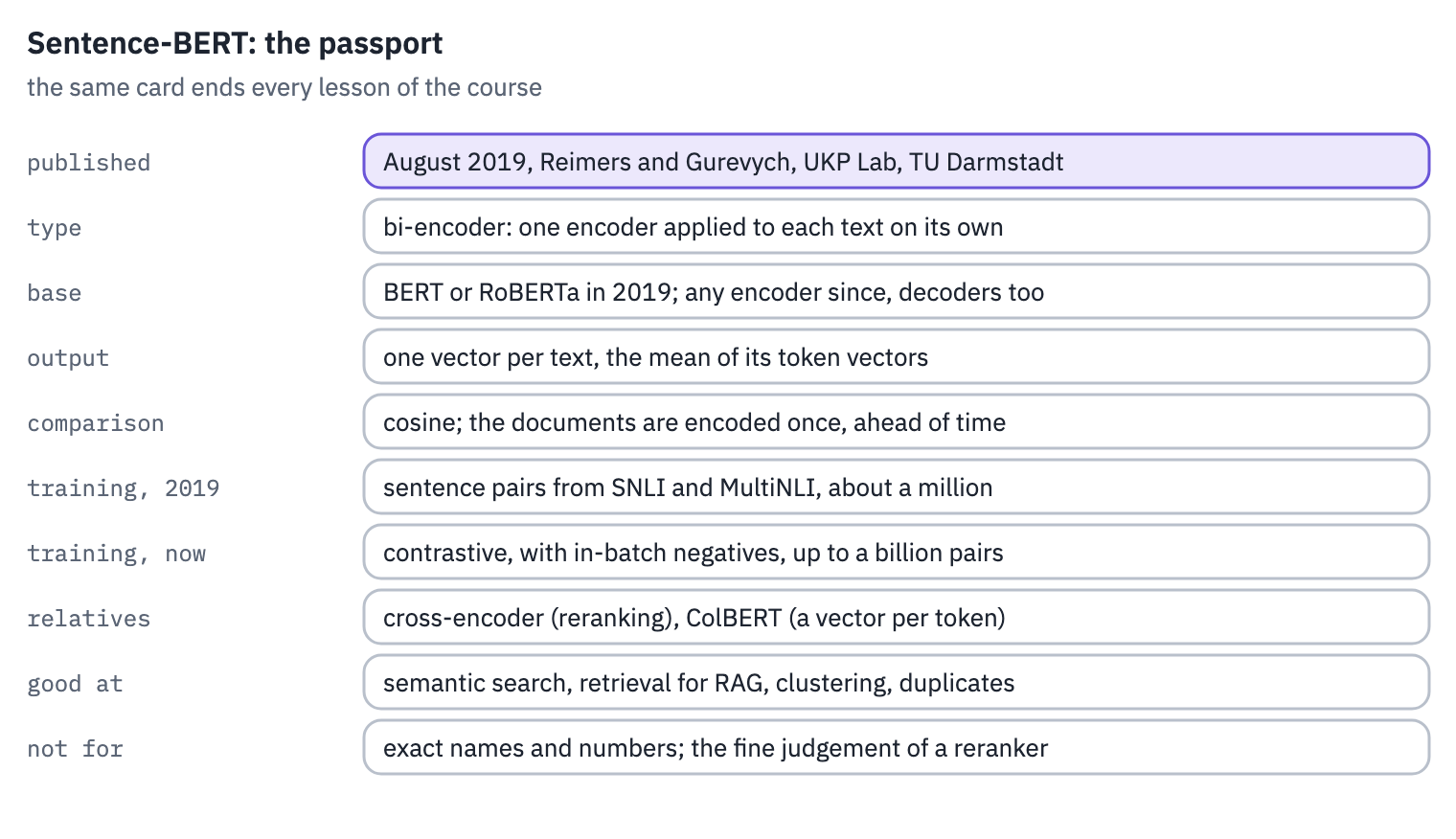
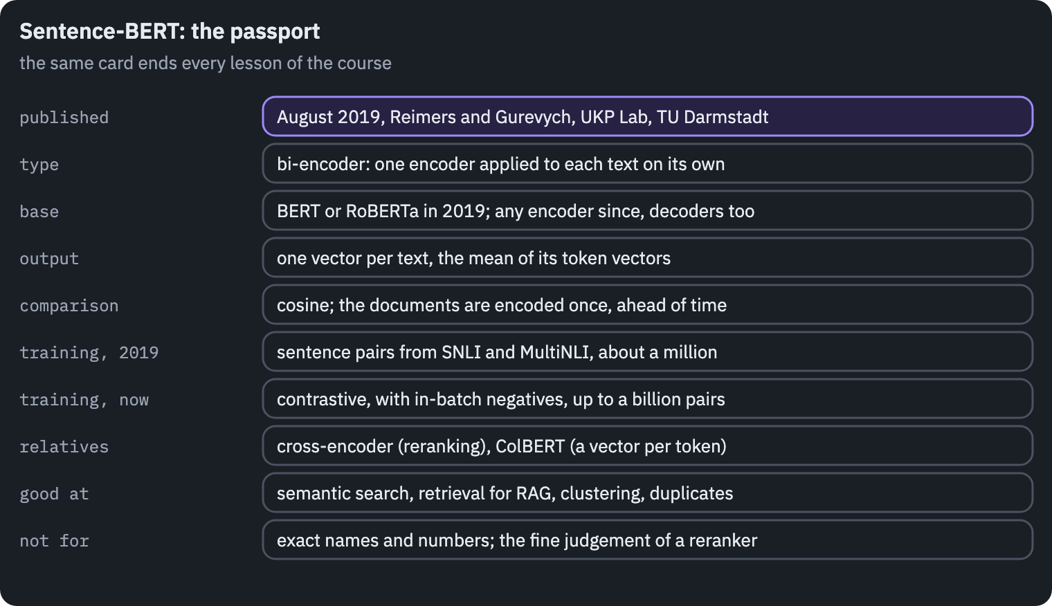
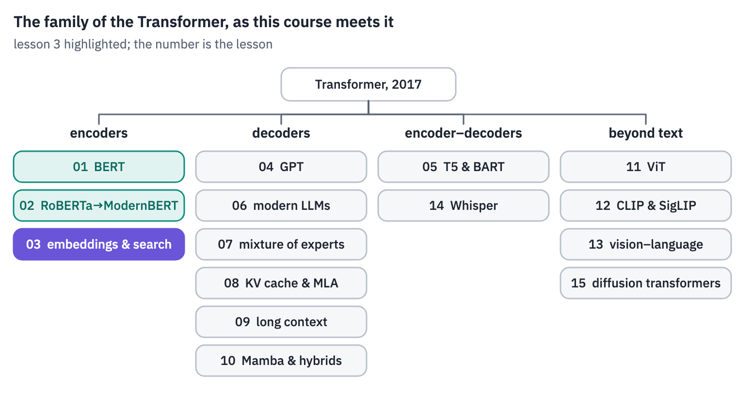
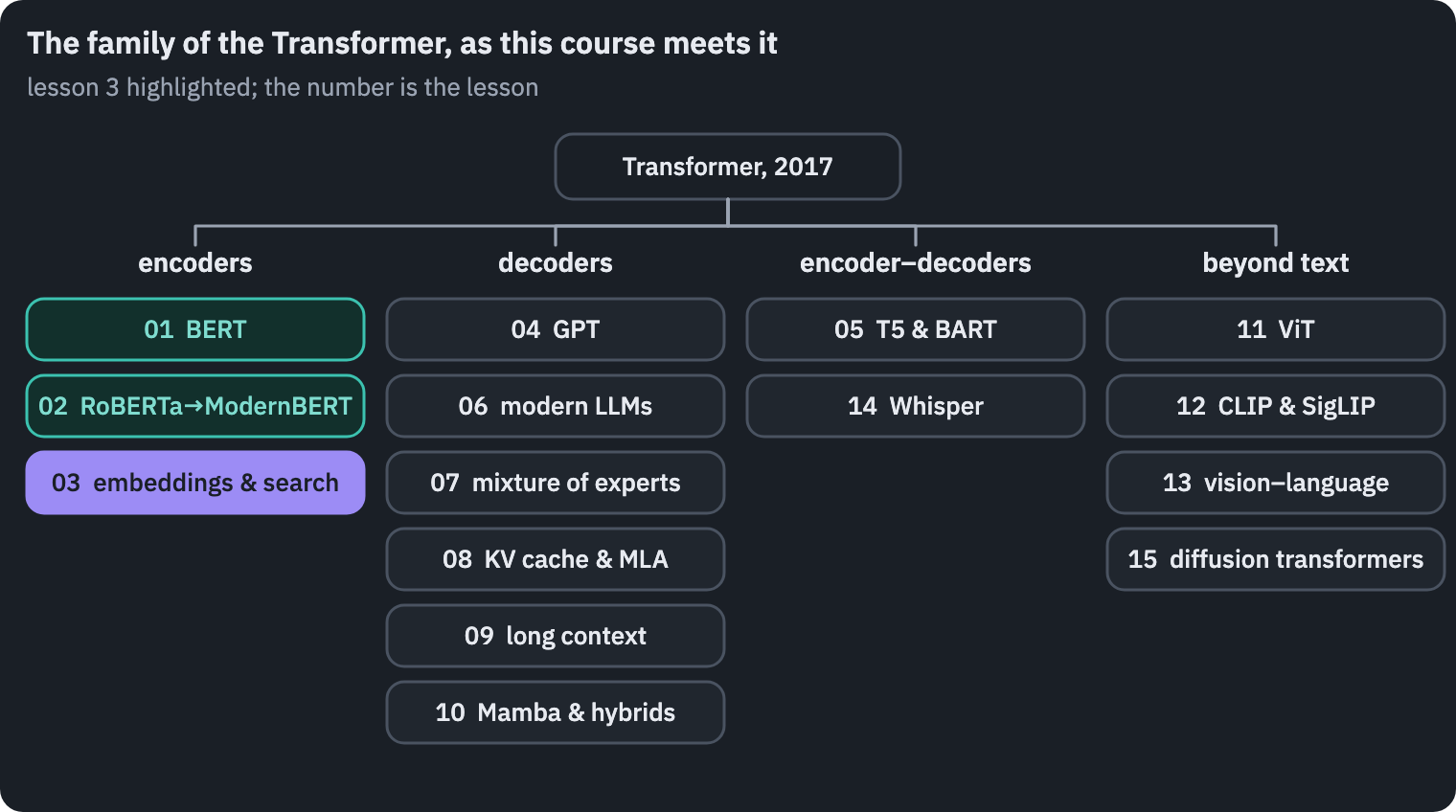
Sentence-BERT’s passport, and the family tree with this lesson’s branch:
References
- Reimers, N., & Gurevych, I. (2019). Sentence-BERT: sentence embeddings using Siamese BERT-networks. EMNLP-IJCNLP 2019. ↩
- Ajith, A., Xia, M., Chevalier, A., Goyal, T., Chen, D., & Gao, T. (2024). LitSearch: a retrieval benchmark for scientific literature search. EMNLP 2024. ↩
- Robertson, S. E., Walker, S., Jones, S., Hancock-Beaulieu, M., & Gatford, M. (1995). Okapi at TREC-3. The Third Text REtrieval Conference (TREC-3), NIST SP 500-226. ↩
- Wang, W., Wei, F., Dong, L., Bao, H., Yang, N., & Zhou, M. (2020). MiniLM: deep self-attention distillation for task-agnostic compression of pre-trained transformers. NeurIPS 2020. ↩
- Henderson, M., Al-Rfou, R., Strope, B., Sung, Y., Lukács, L., Guo, R., Kumar, S., Miklos, B., & Kurzweil, R. (2017). Efficient natural language response suggestion for Smart Reply. arXiv:1705.00652. ↩
- Karpukhin, V., Oğuz, B., Min, S., Lewis, P., Wu, L., Edunov, S., Chen, D., & Yih, W. (2020). Dense passage retrieval for open-domain question answering. EMNLP 2020. ↩
- van den Oord, A., Li, Y., & Vinyals, O. (2018). Representation learning with contrastive predictive coding. arXiv:1807.03748. ↩
- Xiao, S., Liu, Z., Zhang, P., Muennighoff, N., Lian, D., & Nie, J.-Y. (2023). C-Pack: packed resources for general Chinese embeddings. SIGIR 2024. ↩
- Nogueira, R., & Cho, K. (2019). Passage re-ranking with BERT. arXiv:1901.04085. ↩
- Khattab, O., & Zaharia, M. (2020). ColBERT: efficient and effective passage search via contextualized late interaction over BERT. SIGIR 2020. ↩
- Santhanam, K., Khattab, O., Saad-Falcon, J., Potts, C., & Zaharia, M. (2022). ColBERTv2: effective and efficient retrieval via lightweight late interaction. NAACL 2022. ↩
- Cormack, G. V., Clarke, C. L. A., & Büttcher, S. (2009). Reciprocal rank fusion outperforms Condorcet and individual rank learning methods. SIGIR 2009. ↩
- Santhanam, K., Khattab, O., Potts, C., & Zaharia, M. (2022). PLAID: an efficient engine for late interaction retrieval. CIKM 2022. ↩
- Muennighoff, N., Tazi, N., Magne, L., & Reimers, N. (2022). MTEB: massive text embedding benchmark. EACL 2023. ↩
- Ethayarajh, K. (2019). How contextual are contextualized word representations? Comparing the geometry of BERT, ELMo, and GPT-2 embeddings. EMNLP-IJCNLP 2019.