PEFT Method Overview [implementing Adapters in PyTorch]
In the rapidly evolving landscape transformer-based architectures, a significant challenge has emerged: how do we customize these increasingly massive models for specific tasks without breaking the bank on computational resources?
Enter Parameter-Efficient Fine-Tuning (PEFT), a family of techniques that has revolutionized how we adapt pre-trained models to downstream tasks.
The Fine-Tuning Dilemma
So, you’ve got access to a SoTA LM with billions of parameters.
Perhaps it’s GPT-4, LLaMA 3, Mistral or Qwen. You want to adapt this model to a specialized domain like medical text analysis or legal document processing.
The traditional approach would involve fine-tuning the entire model on your domain-specific data.
Full fine-tuning comes with substantial costs:
- Computational Expense: Training billions of parameters requires significant GPU resources.
- Storage Overhead: Each fine-tuned version requires storing a complete copy of the model
- Catastrophic Forgetting: Aggressive fine-tuning might cause the model to lose its general capabilities
- Limited Scalability: Maintaining multiple specialized versions becomes unmanageable
This is where PEFT techniques come to the rescue. Rather than updating all parameters, PEFT methods focus on adding and training a small number of parameters while keeping most of the pre-trained model frozen. This approach typically requires updating less than 1% of the parameters compared to full fine-tuning, while achieving comparable performance.
Let’s understand most significant PEFT methods, their core principles, and implement them using PyTorch for better understanding. Then we’ll explore how to use these techniques with the Hugging Face peft library for practical applications.
General Overview of PEFT methods
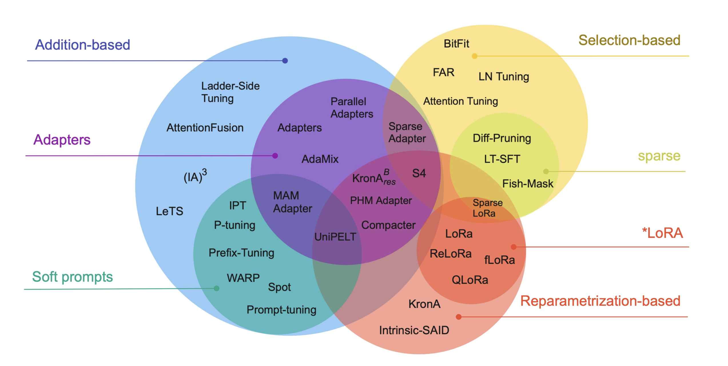
1. Addition-Based Methods
These approaches add new, lightweight modules to a pre-trained model while keeping the original weights frozen. This is the most widely explored category and includes two main subtypes: adapters and soft prompts.
- Adapters (e.g., Bottleneck Adapters, Parallel Adapters): Small neural layers inserted within Transformer blocks that are trained while the rest of the model remains unchanged. Variants differ in placement, structure, and compression strategies.
- LoRA (Low-Rank Adaptation): Instead of fine-tuning full weight matrices, LoRA introduces low-rank decompositions for weight updates (e.g., replacing a full-rank update with
W_down * W_up). - Prefix Tuning / Prompt Tuning: Add trainable vectors (prefixes or prompts) to the model’s input or internal layers. These methods steer model behavior without changing its core parameters.
- Soft Prompts: Instead of using discrete tokens, these train continuous embeddings that are prepended to the input. Can be applied to input embeddings or even across all Transformer layers.
Despite adding new parameters, these methods often use significantly less memory and are more computationally efficient due to fewer gradients and optimizer states being updated.
2. Selection-Based Methods
Selective approaches involve fine-tuning only a specific subset of the model’s original parameters, chosen either manually or via structural criteria.
- BitFit: Fine-tunes only the bias terms of the model, drastically reducing the number of parameters involved.
- IA³ (Infused Adapter by Inhibiting and Amplifying Activations): Adds scalar gating parameters to control the flow of information through the attention and feed-forward layers.
- Layer-wise Selection: Fine-tunes only the top or bottom layers of the model, or focuses on specific components (e.g., attention vs. FFN).
- Sparse Fine-Tuning: Selects parameters to update based on certain criteria (e.g., magnitude or gradients), ignoring model structure. However, this poses practical challenges for current hardware.
These methods are particularly useful when model updates must be extremely lightweight or constrained due to storage, bandwidth, or privacy concerns.
3. Reparameterization-Based Methods
These techniques re-structure the parameter space to enable efficient updates with fewer trainable weights.
- LoRA (also fits here): Uses low-rank matrices to model weight updates, greatly reducing parameter count.
- Compacter: Builds on adapters but compresses them using low-rank decomposition and parameter sharing.
- (IA)³: Combines gating and reparameterization ideas to modulate specific subcomponents of the model.
- KronA / Kron Adapter: Uses Kronecker product decomposition to represent weight updates with a favorable trade-off between expressiveness and size.
- Intrinsic SAID: Employs the Fastfood transform to apply updates within a low-rank subspace, based on the theory that fine-tuning operates within a lower-dimensional manifold.
These methods often target attention-related weights like W_Q, W_K, W_V, where much of the model’s representational power lies.
4. Hybrid Methods
Hybrid approaches combine strategies from multiple categories to balance trade-offs in memory, compute, and performance.
- MAM Adapter: Combines Adapters with Prompt Tuning for better modularity.
- UniPELT: Merges LoRA with Adapters and Prompts into a unified framework.
- Compacter++ / Kron Adapter: Combines adapter-based methods with Kronecker reparameterization to reduce the number of trainable parameters further.
These methods allow researchers to adapt fine-tuning strategies to specific deployment constraints, whether that be edge devices, multi-task learning, or multilingual models.
Bottleneck Adapters
Adapters were among the first successful PEFT approaches, introduced in Parameter-Efficient Transfer Learning for NLP by Houlsby et al. in 2019.
The core idea is elegantly simple: insert small trainable modules into each layer of a pre-trained network while keeping the original parameters frozen.
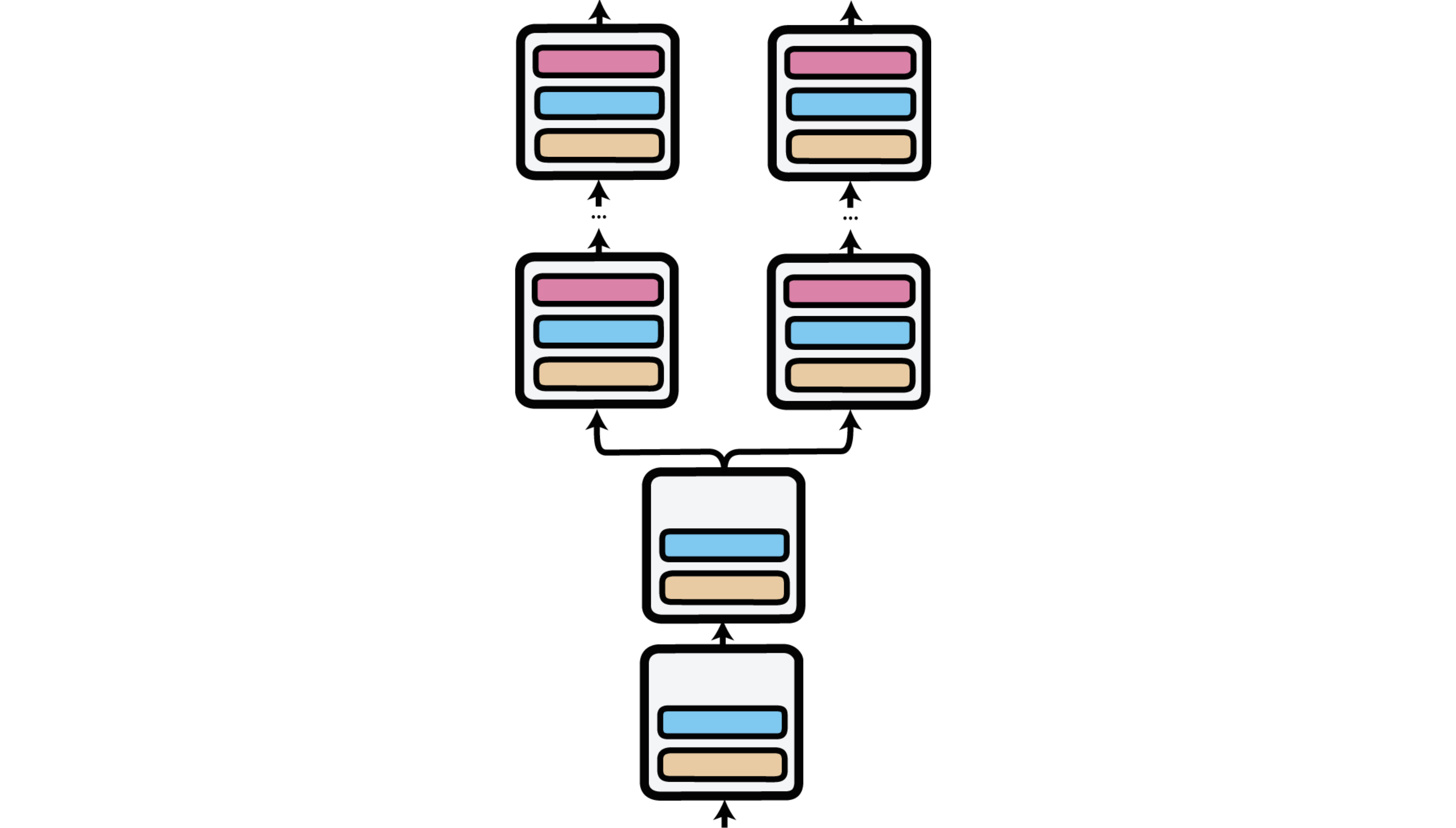
Bottleneck adapters add lightweight feed-forward layers into each Transformer block. These adapter layers typically include:
- a down-projection matrix that reduces the hidden state dimension from \(d\) to a smaller dimension \(b\),
- a non-linear activation \(\sigma\),
- an up-projection matrix that expands the representation back to the original size \(d\), and
- a residual connection, so the original input is added back after transformation:
Depending on the specific configuration, these adapter layers can be placed at various points inside the Transformer block. Other components like residual connections, layer normalizations, activation functions, and the size of the bottleneck layer can also be customized.
The most important hyperparameter in this setup is the bottleneck dimension \(b\). Rather than setting \(b\) directly, it’s usually defined through a parameter called reduction_factor. This factor represents the ratio between the hidden layer size \(d\) and the bottleneck size \(b\), given by:
class BottleneckAdapter(nn.Module):
    def __init__(self, hidden_size, adapter_size, dropout_rate=0.1):
        """
        A bottleneck adapter module that can be inserted into a transformer.

        It projects hidden states down to a lower-dimensional space and then
        back up again, with non-linearity and dropout in between. This helps
        the model adapt to new tasks without updating the original transformer.

        Args:
            hidden_size: The dimension of the model's hidden states (e.g., 768 for BERT-base)
            adapter_size: The smaller bottleneck dimension (e.g., 64)
            dropout_rate: Regularization to improve generalization
        """
        super().__init__()

        self.down_project = nn.Linear(hidden_size, adapter_size)  # d -> b
        self.activation = nn.GELU()  # non-linearity
        self.up_project = nn.Linear(adapter_size, hidden_size)    # b -> d
        self.dropout = nn.Dropout(dropout_rate)
        self.layer_norm = nn.LayerNorm(hidden_size)

        # Initialize adapter weights — not learned from pretraining, so good init is important!
        nn.init.xavier_uniform_(self.down_project.weight)
        nn.init.zeros_(self.down_project.bias)
        nn.init.xavier_uniform_(self.up_project.weight)
        nn.init.zeros_(self.up_project.bias)

    def forward(self, hidden_states):
        # Store original input for residual connection
        residual = hidden_states

        # Apply adapter: down-project -> non-linear -> up-project -> dropout
        x = self.down_project(hidden_states)
        x = self.activation(x)
        x = self.up_project(x)
        x = self.dropout(x)

        # Add residual and normalize
        output = residual + x
        output = self.layer_norm(output)
        return output
But how do we integrate adapters into a pre-trained model?
Let’s see how to modify a standard transformer layer to include our bottleneck adapter:
class AdapterTransformerLayer(nn.Module):
    def __init__(self, transformer_layer, adapter_size):
        """
        A wrapper around an existing transformer layer that adds adapters after
        attention and after the feed-forward sublayers.

        Args:
            transformer_layer: One layer from a pre-trained transformer (e.g., BERTLayer)
            adapter_size: Bottleneck size for the adapters
        """
        super().__init__()
        self.layer = transformer_layer
        self.hidden_size = transformer_layer.attention.self.all_head_size  # Model-specific

        # Freeze all transformer weights (we don’t train them)
        for param in self.layer.parameters():
            param.requires_grad = False

        # Add bottleneck adapters at two key places:
        self.attention_adapter = BottleneckAdapter(self.hidden_size, adapter_size)
        self.ffn_adapter = BottleneckAdapter(self.hidden_size, adapter_size)

    def forward(self, hidden_states, attention_mask=None):
        # Standard attention (output of frozen pre-trained layer)
        attention_output = self.layer.attention(hidden_states, attention_mask)[0]

        # Inject adapter after attention
        adapted_attention = self.attention_adapter(attention_output)

        # Apply frozen feed-forward network
        intermediate_output = self.layer.intermediate(adapted_attention)
        layer_output = self.layer.output(intermediate_output, adapted_attention)

        # Inject second adapter after feed-forward
        output = self.ffn_adapter(layer_output)

        return output
All set, and we need to load pre-trained model and wrap it’s target layers with this.
model = BertModel.from_pretrained("bert-base-uncased")
tokenizer = BertTokenizer.from_pretrained("bert-base-uncased")

# Define adapter size
adapter_size = 64

# Wrap all encoder layers with adapter-enabled versions
for i in range(len(model.encoder.layer)):
    original_layer = model.encoder.layer[i]
    model.encoder.layer[i] = AdapterTransformerLayer(original_layer, adapter_size)
# Check that only adapters will be trained
trainable_params = sum(p.numel() for p in model.parameters() if p.requires_grad)
total_params = sum(p.numel() for p in model.parameters())
print(f"Trainable parameters: {trainable_params} / {total_params}")

# Now you can tokenize input and train like usual.
inputs = tokenizer("Adapters are lightweight and powerful.", return_tensors="pt")
outputs = model(**inputs)
Now, I’m gonna show how to use adapters in transformers library. It’s faster, easier, and production-tested.
# pip install adapter-transformers

# `BertAdapterModel` = a special version of BERT that allows adapter injection.
from transformers import BertTokenizer, BertAdapterModel
from transformers.adapters import AdapterConfig

# Load model and tokenizer
tokenizer = BertTokenizer.from_pretrained("bert-base-uncased")
model = BertAdapterModel.from_pretrained("bert-base-uncased")

# Define adapter configuration
config = AdapterConfig.load(
    "pfeiffer",                    # Adapter type: "pfeiffer", "houlsby", etc.
    reduction_factor=16,          # Bottleneck size (768 / 16 = 48)
    leave_out=[0, 11],            # Skip layer 0 and 11 (i.e., don't inject there)
    non_linearity="gelu",
)

# Add adapter with a custom name
model.add_adapter("my_task_adapter", config=config)

# Activate + train this adapter
model.train_adapter("my_task_adapter")

#Tokenize Input and Forward Pass
inputs = tokenizer("Adapters are efficient!", return_tensors="pt")
outputs = model(**inputs)

# Last hidden state (batch_size, seq_len, hidden_dim)
print(outputs.last_hidden_state.shape)

# Add a Classification Head (for downstream tasks)
model.add_classification_head("my_task_adapter", num_labels=2)

# Switch to training mode
model.train_adapter("my_task_adapter")

# Forward pass for classification
inputs = tokenizer("Adapters are awesome!", return_tensors="pt")
outputs = model(**inputs)
logits = outputs.logits

# Training Only Adapter Parameters
optimizer = torch.optim.Adam(filter(lambda p: p.requires_grad, model.parameters()), lr=5e-5)

# Save / Load Adapters Separately

# Save adapter after training
model.save_adapter("saved/my_task_adapter", "my_task_adapter")

# Load later into another model
model.load_adapter("saved/my_task_adapter", load_as="my_task_adapter")
model.set_active_adapters("my_task_adapter")
Parallel Adapters
While bottleneck adapters are inserted sequentially in the model’s architecture, parallel Adapters inject adapter modules in parallel with the main feed-forward layers in each Transformer block, instead of sequentially. This means that the output of the adapter is added to the output of the feed-forward network, not to its input.
Let \(x\) be the input to the Transformer block. The original feed-forward output is \(\mathrm{FFN}(x)\), and the adapter path is:
\[\mathrm{Adapter}(x) = W_\text{up} \, \sigma(W_\text{down} \, x)\]The final output becomes:
\[y = \mathrm{FFN}(x) + \mathrm{Adapter}(x)\]This allows the adapter to independently learn task-specific modifications without disrupting the main path.
The parallel design has a slight computational overhead but can better preserve the pre-trained representations.
class ParallelAdapter(nn.Module):
    def __init__(self, hidden_size, adapter_size, dropout_rate=0.1):
        super().__init__()
        self.down_project = nn.Linear(hidden_size, adapter_size)
        self.activation = nn.GELU()
        self.up_project = nn.Linear(adapter_size, hidden_size)
        self.dropout = nn.Dropout(dropout_rate)

        # Initialize weights
        nn.init.xavier_uniform_(self.down_project.weight)
        nn.init.zeros_(self.down_project.bias)
        nn.init.xavier_uniform_(self.up_project.weight)
        nn.init.zeros_(self.up_project.bias)

        # Scale factor - can be trained or fixed
        self.scaling_factor = nn.Parameter(torch.tensor(0.1))

    def forward(self, hidden_states):
        x = self.down_project(hidden_states)
        x = self.activation(x)
        x = self.up_project(x)
        x = self.dropout(x)

        # Scale the adapter output and add to original
        return hidden_states + self.scaling_factor * x
The integration into a transformer layer would be similar to the bottleneck adapter, but the adapter would be applied in parallel rather than sequentially.
Low-Rank Adaptation (LoRA)
LoRA (Low-Rank Adaptation) introduced by Hu et al. (2021) replaces or augments weight matrices with low-rank decompositions. Instead of fine-tuning a full matrix \(W \in \mathbb{R}^{d \times d}\), LoRA learns two smaller matrices:
\[W' = W + A B \quad \text{with} \quad A \in \mathbb{R}^{d \times r}, \; B \in \mathbb{R}^{r \times d}\]Where \(r \ll d\) (typically \(r = 8\) or \(4\)). This drastically reduces the number of trainable parameters. LoRA is usually applied to the attention projection layers (query/key/value/output).
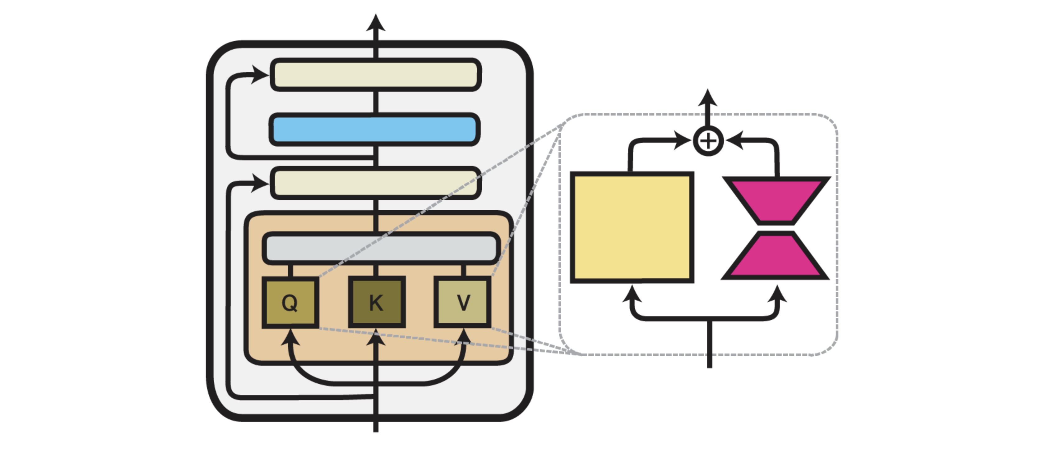
Intuitively, LoRA adds a “low-rank path” through which task-specific information can flow, while keeping the rest of the model fixed.
class LoRALayer(nn.Module):
    def __init__(self, in_features, out_features, rank=8, alpha=32):
        """
        LoRA implementation for linear layers.

        Args:
            in_features: Input dimension
            out_features: Output dimension
            rank: Rank of the low-rank decomposition
            alpha: Scaling factor for the LoRA contribution
        """
        super().__init__()
        self.rank = rank
        self.scaling = alpha / rank

        # LoRA weights
        self.lora_A = nn.Parameter(torch.zeros(in_features, rank))
        self.lora_B = nn.Parameter(torch.zeros(rank, out_features))

        # Initialize weights
        nn.init.kaiming_uniform_(self.lora_A, a=math.sqrt(5))
        nn.init.zeros_(self.lora_B)

    def forward(self, x):
        # LoRA contribution: scaling * (x @ A) @ B
        return self.scaling * (x @ self.lora_A) @ self.lora_B
Now, let’s apply LoRA to a pre-trained linear layer:
class LoRALinear(nn.Module):
    def __init__(self, linear_layer, rank=8, alpha=32):
        """
        Wraps a pre-trained linear layer with LoRA functionality.

        Args:
            linear_layer: The pre-trained nn.Linear module to adapt
            rank: Rank of the low-rank decomposition
            alpha: Scaling factor
        """
        super().__init__()
        self.linear = linear_layer

        # Freeze original weights
        self.linear.weight.requires_grad = False
        if self.linear.bias is not None:
            self.linear.bias.requires_grad = False

        # Add LoRA components
        self.lora = LoRALayer(
            linear_layer.in_features,
            linear_layer.out_features,
            rank=rank,
            alpha=alpha
        )

    def forward(self, x):
        # Combine original output with LoRA contribution
        return self.linear(x) + self.lora(x)
The genius of LoRA is in its efficiency.
If the original weight matrix has dimensions n×m, full fine-tuning would require updating n×m parameters. With LoRA, using a rank r, we only need to update r×(n+m) parameters. For large matrices where r « min(n,m), this represents a massive reduction in trainable parameters.
Applying LoRA to a Transformer
In practice, LoRA is typically applied to specific weight matrices within a transformer, most commonly the query and value projection matrices in attention layers. Here’s how to adapt a transformer’s attention mechanism with LoRA:
import math
from transformers import AutoModel

def apply_lora_to_model(model, rank=8, alpha=32, target_modules=["q_proj", "v_proj"]):
    """
    Apply LoRA to specific modules in a transformer model.

    Args:
        model: A Hugging Face transformer model
        rank: Rank for LoRA decomposition
        alpha: Scaling factor
        target_modules: List of module names to apply LoRA to
    """
    # First, freeze all parameters
    for param in model.parameters():
        param.requires_grad = False

    # Then apply LoRA to target modules
    for name, module in model.named_modules():
        if any(target_name in name for target_name in target_modules):
            if isinstance(module, nn.Linear):
                # Get the parent module
                parent_name = '.'.join(name.split('.')[:-1])
                child_name = name.split('.')[-1]
                parent_module = model.get_submodule(parent_name)

                # Replace with LoRA version
                lora_layer = LoRALinear(module, rank=rank, alpha=alpha)
                setattr(parent_module, child_name, lora_layer)

    return model

model = AutoModel.from_pretrained("bert-base-uncased")
lora_model = apply_lora_to_model(model)
Quantized LoRA (QLoRA)
QLoRA, takes LoRA’s efficiency to the next level by combining it with quantization techniques. The key insight is to keep the base model in a quantized format (typically 4-bit precision) while applying LoRA adapters in full precision.
QLoRA has been a game-changer for democratizing LLM fine-tuning, enabling the adaptation of models with over 70 billion parameters on a single consumer GPU.
Prefix Tuning: Virtual Tokens in Hidden Space
Now let’s shift our focus to another family of PEFT methods that operate by introducing trainable tokens to the input sequence or hidden states: Prefix Tuning and Prompt Tuning.
Prefix Tuning, introduced by Li and Liang (2021), prepends a small number of learned key-value vectors (“prefixes”) to the attention mechanism.
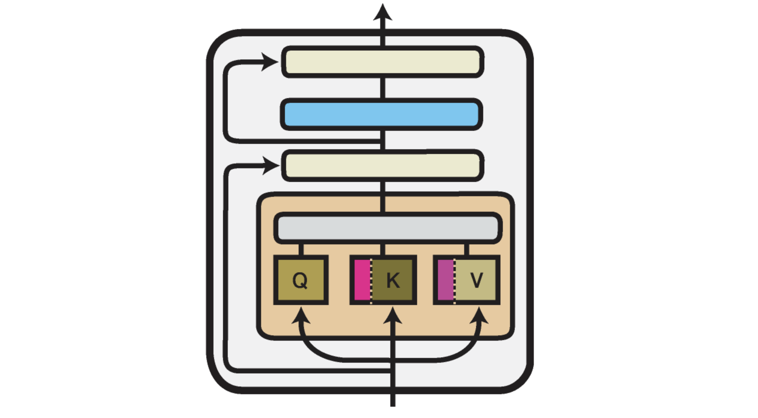
Instead of modifying weights, it expands the input to attention as:
\[\text{Attention}(\text{prefix} + x)\]This means the model sees the learned prefix as a pseudo-context for every input, influencing the attention output without changing the underlying Transformer parameters.
Prefix tuning is powerful for generation tasks like summarization or translation where modifying the attention context is sufficient.
class PrefixTuningModule(nn.Module):
    def __init__(self, hidden_size, prefix_length=20, num_layers=12, num_heads=12, head_dim=64):
        """
        Implementation of Prefix Tuning.

        Args:
            hidden_size: Model's hidden size
            prefix_length: Number of virtual tokens to add
            num_layers: Number of transformer layers
            num_heads: Number of attention heads
            head_dim: Dimension of each attention head
        """
        super().__init__()
        self.prefix_length = prefix_length
        self.num_layers = num_layers
        self.num_heads = num_heads
        self.head_dim = head_dim

        # Create a prefix for each layer for both key and value states
        # Shape: [num_layers, 2, prefix_length, num_heads, head_dim]
        self.prefix_tokens = nn.Parameter(
            torch.zeros(num_layers, 2, prefix_length, num_heads, head_dim)
        )

        # Initialize with a small standard deviation
        nn.init.normal_(self.prefix_tokens, std=0.02)

    def forward(self, key_value_states, layer_idx):
        """
        Prepend prefix to key and value states for a specific layer.

        Args:
            key_value_states: Tuple of (key, value) states from the model
            layer_idx: Current transformer layer index
        """
        key_states, value_states = key_value_states
        batch_size = key_states.shape[0]

        # Get the prefix for the current layer
        # Shape: [2, prefix_length, num_heads, head_dim]
        prefix = self.prefix_tokens[layer_idx]

        # Extract key and value prefixes
        key_prefix = prefix[0].expand(batch_size, -1, -1, -1)
        value_prefix = prefix[1].expand(batch_size, -1, -1, -1)

        # Reshape to match model's key and value shapes
        # From: [batch_size, prefix_length, num_heads, head_dim]
        # To: [batch_size, num_heads, prefix_length, head_dim]
        key_prefix = key_prefix.permute(0, 2, 1, 3)
        value_prefix = value_prefix.permute(0, 2, 1, 3)

        # Concatenate with original states
        # Original shape: [batch_size, num_heads, seq_length, head_dim]
        new_key_states = torch.cat([key_prefix, key_states], dim=2)
        new_value_states = torch.cat([value_prefix, value_states], dim=2)

        return (new_key_states, new_value_states)
To integrate this with a transformer model, we need to modify each attention layer to incorporate the prefixes:
class PrefixTransformerLayer(nn.Module):
    def __init__(self, transformer_layer, prefix_module, layer_idx):
        super().__init__()
        self.layer = transformer_layer
        self.prefix_module = prefix_module
        self.layer_idx = layer_idx

        # Freeze the original layer
        for param in self.layer.parameters():
            param.requires_grad = False

    def forward(self, hidden_states, attention_mask=None):
        # Extract the attention module (implementation depends on model architecture)
        attention = self.layer.attention.self

        # Prepare key, query, value states as in the original attention
        query_states = attention.query(hidden_states)
        key_states = attention.key(hidden_states)
        value_states = attention.value(hidden_states)

        # Reshape for multi-head attention
        batch_size, seq_length = hidden_states.shape[:2]
        head_dim = attention.head_size
        num_heads = attention.num_attention_heads

        query_states = query_states.view(batch_size, seq_length, num_heads, head_dim).transpose(1, 2)
        key_states = key_states.view(batch_size, seq_length, num_heads, head_dim).transpose(1, 2)
        value_states = value_states.view(batch_size, seq_length, num_heads, head_dim).transpose(1, 2)

        # Apply prefix
        key_states, value_states = self.prefix_module((key_states, value_states), self.layer_idx)

        # Update attention mask for the additional prefix tokens
        if attention_mask is not None:
            prefix_attention_mask = torch.ones(
                batch_size,
                1,
                1,
                self.prefix_module.prefix_length,
                device=attention_mask.device
            )
            extended_attention_mask = torch.cat([prefix_attention_mask, attention_mask], dim=-1)
        else:
            extended_attention_mask = None

        # Calculate attention scores and outputs
        # (Implementation depends on the specific attention mechanism)
        # ...

        return output
The above implementation is conceptual and would need to be adapted based on the specific transformer architecture you’re working with.
Prompt Tuning
Prompt Tuning, can be seen as a simplified version of Prefix Tuning. Rather than adding virtual tokens at every layer, Prompt Tuning only prepends trainable embeddings to the input sequence embeddings at the first layer.
Here’s a straightforward implementation:
class PromptTuning(nn.Module):
    def __init__(self, model, prompt_length=20):
        """
        Implementation of Prompt Tuning.

        Args:
            model: The pre-trained transformer model
            prompt_length: Number of virtual tokens to add
        """
        super().__init__()
        self.model = model
        self.prompt_length = prompt_length

        # Freeze model parameters
        for param in model.parameters():
            param.requires_grad = False

        # Get embedding dimension from the model
        embed_dim = model.get_input_embeddings().weight.shape[1]

        # Create soft prompt embeddings
        self.soft_prompts = nn.Parameter(torch.randn(prompt_length, embed_dim))

        # Initialize with embeddings of random tokens from the vocabulary
        with torch.no_grad():
            vocab_size = model.get_input_embeddings().weight.shape[0]
            random_indices = torch.randint(0, vocab_size, (prompt_length,))
            self.soft_prompts.data = model.get_input_embeddings().weight[random_indices].clone()

    def forward(self, input_ids=None, attention_mask=None, **kwargs):
        batch_size = input_ids.shape[0] if input_ids is not None else attention_mask.shape[0]

        # Get input embeddings
        if input_ids is not None:
            inputs_embeds = self.model.get_input_embeddings()(input_ids)
        else:
            inputs_embeds = kwargs.pop("inputs_embeds")

        # Expand soft prompts for batch size and prepend to input embeddings
        prompt_embeds = self.soft_prompts.unsqueeze(0).expand(batch_size, -1, -1)
        inputs_embeds = torch.cat([prompt_embeds, inputs_embeds], dim=1)

        # Adjust attention mask for the added prompt tokens
        if attention_mask is not None:
            prompt_mask = torch.ones(batch_size, self.prompt_length, device=attention_mask.device)
            attention_mask = torch.cat([prompt_mask, attention_mask], dim=1)

        # Forward pass through the model without input_ids
        return self.model(
            input_ids=None,
            attention_mask=attention_mask,
            inputs_embeds=inputs_embeds,
            **kwargs
        )
BitFit Adapter
BitFit, proposed by Zaken et al. (2021), takes a radically different approach from the methods we’ve discussed so far. Instead of adding new parameters, BitFit selectively trains only the bias terms in the pre-trained model, leaving all other parameters frozen.
Despite its extreme parameter efficiency, BitFit has shown good performance across various tasks.
def apply_bitfit_to_model(model):
    """
    Apply BitFit to a transformer model by only training bias terms.

    Args:
        model: A PyTorch model
    """
    # First, freeze all parameters
    for param in model.parameters():
        param.requires_grad = False

    # Then unfreeze only bias parameters
    for name, param in model.named_parameters():
        if "bias" in name:
            param.requires_grad = True

    return model
The implementation is remarkably simple, yet BitFit can achieve competitive performance while training less than 0.1% of the original model parameters in many cases.
IA³: Infused Adapter by Inhibiting and Amplifying Inner Activations
IA³ (Input-Aware Activation Adjustment) by Liu et al. (2022), modifies the element-wise activation scale and bias after each linear transformation. For a layer with output \(x\), IA³ computes:
\[x' = \alpha \cdot x + \beta\]Here, \(\alpha\) and \(\beta\) are trainable parameters. This is similar to fine-tuning just the scale and shift of activations and can be extremely efficient.
IA³ is useful when slight shifts in activation distributions are enough to steer the model to the new task.
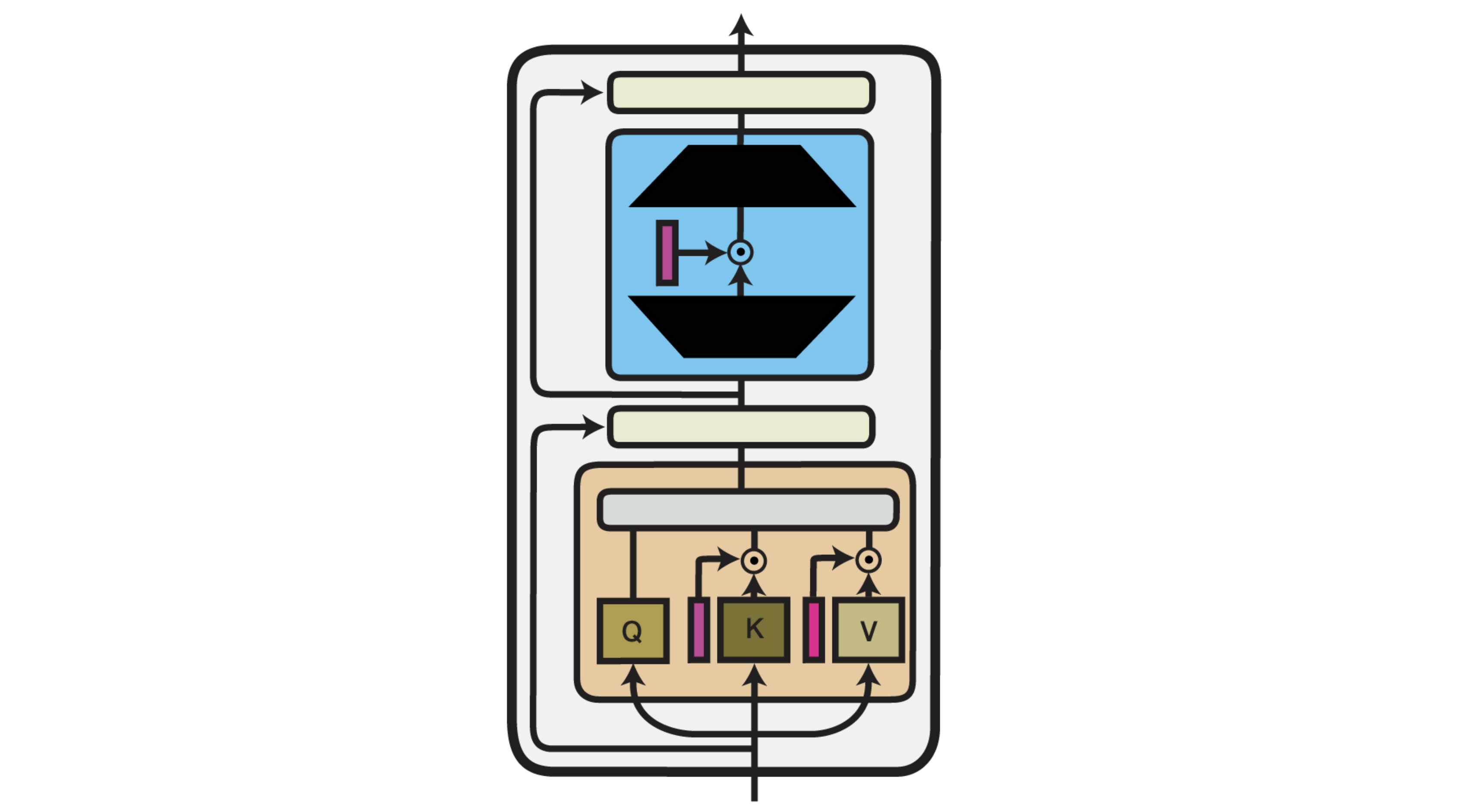
Let’s check how it looks like in the code.
class IA3Module(nn.Module):
    def __init__(self, hidden_size, ia3_type="feed_forward"):
        """
        Implementation of IA³ scaling vectors.

        Args:
            hidden_size: Dimension to scale
            ia3_type: Where to apply IA³ ('feed_forward', 'attention_output', 'attention_value')
        """
        super().__init__()
        self.ia3_type = ia3_type

        # Create scaling vectors initialized to ones
        if ia3_type == "feed_forward":
            # For the output of the feed-forward layer
            self.scaling_vector = nn.Parameter(torch.ones(hidden_size))
        elif ia3_type == "attention_output":
            # For scaling attention outputs
            self.scaling_vector = nn.Parameter(torch.ones(hidden_size))
        elif ia3_type == "attention_value":
            # For scaling value vectors in attention
            self.scaling_vector = nn.Parameter(torch.ones(hidden_size))

    def forward(self, x):
        """
        Apply scaling to input tensor.
        """
        if self.ia3_type == "attention_value":
            # For attention values, we reshape for broadcasting across batch and seq dimensions
            return x * self.scaling_vector.view(1, 1, 1, -1)
        else:
            # For feed-forward and attention outputs
            return x * self.scaling_vector
Integrating IA³ with a transformer model requires injecting the scaling at specific points:
class IA3TransformerLayer(nn.Module):
    def __init__(self, transformer_layer, hidden_size):
        super().__init__()
        self.layer = transformer_layer

        # Freeze original parameters
        for param in self.layer.parameters():
            param.requires_grad = False

        # Add IA³ modules
        self.attention_value_ia3 = IA3Module(hidden_size, ia3_type="attention_value")
        self.attention_output_ia3 = IA3Module(hidden_size, ia3_type="attention_output")
        self.feed_forward_ia3 = IA3Module(hidden_size, ia3_type="feed_forward")

    def forward(self, hidden_states, attention_mask=None):
        # Extract components (implementation is model-specific)
        attention = self.layer.attention.self

        # Compute query, key, value projections
        query = attention.query(hidden_states)
        key = attention.key(hidden_states)
        value = attention.value(hidden_states)

        # Apply IA³ to value projections
        value = self.attention_value_ia3(value)

        # Compute attention
        attention_output = attention(hidden_states, attention_mask)[0]

        # Apply IA³ to attention output
        attention_output = self.attention_output_ia3(attention_output)

        # Feed-forward network
        intermediate_output = self.layer.intermediate(attention_output)
        layer_output = self.layer.output(intermediate_output, attention_output)

        # Apply IA³ to feed-forward output
        output = self.feed_forward_ia3(layer_output)

        return output
IA³’s efficiency is remarkable: for a model with hidden size h, it adds only 3h parameters per layer, compared to the millions in the original layer.
Compacter: Kronecker Products for Ultimate Efficiency
Compacter, proposed by Mahabadi et al. (2021), builds on the adapter idea, but instead of learning full matrices for down/up projection, it composes them from Kronecker products of smaller matrices.
\[W = W_1 \otimes W_2\]This gives an expressive yet parameter-efficient formulation. Compacter adapters can learn more complex transformations than simple low-rank matrices without adding much overhead.
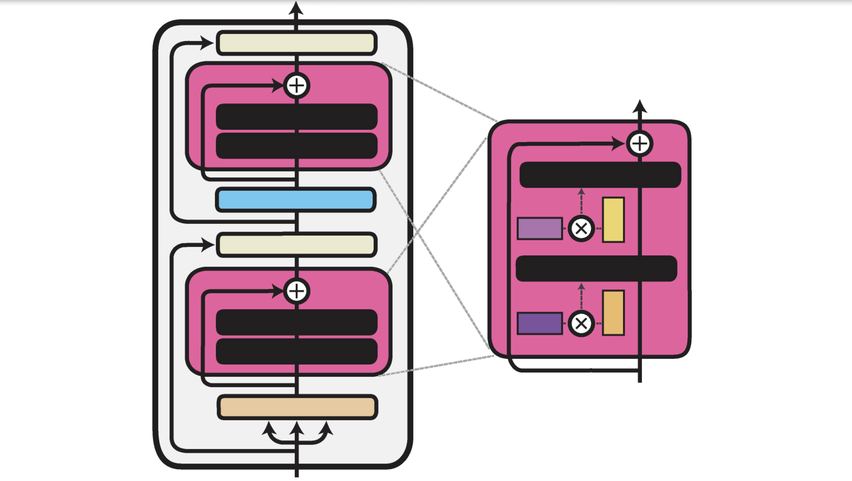
Let’s implement Compacter:
class PHM(nn.Module):
    """
    Parameterized Hypercomplex Multiplication using Kronecker products.
    """
    def __init__(self, in_features, out_features, rank=4, factorized_phm=True):
        super().__init__()
        self.in_features = in_features
        self.out_features = out_features
        self.rank = rank
        self.factorized_phm = factorized_phm

        # Calculate dimensions for the factors
        self.in_factor_size = int(math.sqrt(in_features))
        self.out_factor_size = int(math.sqrt(out_features))

        # Ensure dimensions are compatible with factorization
        assert self.in_factor_size * self.in_factor_size == in_features, \
            "Input features must be a perfect square for factorization"
        assert self.out_factor_size * self.out_factor_size == out_features, \
            "Output features must be a perfect square for factorization"

        if factorized_phm:
            # Factorized representation using shared factors
            self.A = nn.Parameter(torch.empty(rank, self.in_factor_size, self.out_factor_size))
            self.B = nn.Parameter(torch.empty(rank, self.in_factor_size, self.out_factor_size))
        else:
            # Full Kronecker factors
            self.W = nn.Parameter(torch.empty(rank, in_features, out_features))

        self.s = nn.Parameter(torch.ones(rank))

        # Initialize parameters
        self._init_parameters()

    def _init_parameters(self):
        """Initialize the parameters with small random values."""
        if self.factorized_phm:
            nn.init.normal_(self.A, mean=0.0, std=0.02)
            nn.init.normal_(self.B, mean=0.0, std=0.02)
        else:
            nn.init.normal_(self.W, mean=0.0, std=0.02)

        nn.init.ones_(self.s)

    def kronecker_product(self, A, B):
        """
        Compute the Kronecker product of matrices A and B.
        """
        batch_size = A.size(0)
        s1, s2 = A.size(1), A.size(2)
        s3, s4 = B.size(1), B.size(2)

        # Reshape for matrix multiplication
        A_reshaped = A.view(batch_size, s1 * s2, 1)
        B_reshaped = B.view(batch_size, 1, s3 * s4)

        # Perform outer product
        kron_prod = torch.bmm(A_reshaped, B_reshaped)

        # Reshape to get the final Kronecker product
        return kron_prod.view(batch_size, s1, s2, s3, s4).view(batch_size, s1 * s3, s2 * s4)

    def forward(self, x):
        """
        Forward pass using PHM.
        x: Input tensor of shape [batch_size, in_features]
        """
        batch_size = x.size(0)

        # Compute the weight matrix using PHM
        if self.factorized_phm:
            # Using factorized representation
            weight = 0
            for r in range(self.rank):
                # Apply scaling factor
                kronecker_factor = self.kronecker_product(
                    self.A[r].unsqueeze(0).repeat(batch_size, 1, 1),
                    self.B[r].unsqueeze(0).repeat(batch_size, 1, 1)
                )
                weight += self.s[r] * kronecker_factor
        else:
            # Using full representation
            weight = torch.sum(self.W * self.s.view(self.rank, 1, 1), dim=0)

        # Apply the weight matrix - handle factorized vs full differently
        if self.factorized_phm:
            # For factorized version, we already have batch-specific weights
            output = torch.bmm(x.unsqueeze(1), weight).squeeze(1)
        else:
            # For the full version, we use simple matrix multiply
            output = x @ weight

        return output

class CompacterLayer(nn.Module):
    """
    Compacter adapter implementation using PHM for weight parameterization.
    """
    def __init__(self, hidden_size, adapter_size=64, rank=4, factorized_phm=True):
        super().__init__()
        self.hidden_size = hidden_size
        self.adapter_size = adapter_size

        # Down projection using PHM
        self.down_proj = PHM(hidden_size, adapter_size, rank=rank, factorized_phm=factorized_phm)

        # Activation function
        self.activation = nn.GELU()

        # Up projection using PHM
        self.up_proj = PHM(adapter_size, hidden_size, rank=rank, factorized_phm=factorized_phm)

        # Additional components
        self.dropout = nn.Dropout(0.1)
        self.layer_norm = nn.LayerNorm(hidden_size)

        # Scaling factor for the adapter output
        self.scaling_factor = nn.Parameter(torch.tensor(0.1))

    def forward(self, hidden_states):
        """
        Forward pass through the Compacter adapter.
        """
        residual = hidden_states

        # Down projection with PHM
        x = self.down_proj(hidden_states)
        x = self.activation(x)

        # Up projection with PHM
        x = self.up_proj(x)
        x = self.dropout(x)

        # Apply scaling and add residual
        output = residual + self.scaling_factor * x
        output = self.layer_norm(output)

        return output

# Integrating Compacter with a transformer layer would be similar to the adapter implementation
class CompacterTransformerLayer(nn.Module):
    def __init__(self, transformer_layer, adapter_size=64, rank=4):
        super().__init__()
        self.layer = transformer_layer
        hidden_size = transformer_layer.attention.self.all_head_size  # Model specific

        # Freeze original parameters
        for param in self.layer.parameters():
            param.requires_grad = False

        # Add Compacter adapters
        self.attention_adapter = CompacterLayer(hidden_size, adapter_size, rank)
        self.ffn_adapter = CompacterLayer(hidden_size, adapter_size, rank)

    def forward(self, hidden_states, attention_mask=None):
        # Original attention mechanism
        attention_output = self.layer.attention(hidden_states, attention_mask)[0]

        # Apply attention adapter
        adapted_attention = self.attention_adapter(attention_output)

        # Original feed-forward network
        intermediate_output = self.layer.intermediate(adapted_attention)
        layer_output = self.layer.output(intermediate_output, adapted_attention)

        # Apply ffn adapter
        output = self.ffn_adapter(layer_output)

        return output
Enjoy Reading This Article?
Here are some more articles you might like to read next: